---
title: "Checking a biodiversity-function analysis"
description: "Three checks for a biodiversity-ecosystem function partition in R: the monoculture references, additive versus substitutive designs, and one dominant species."
date: "2026-06-29 13:00"
date-modified: "2026-10-15"
categories: [ecology tutorial, R, biodiversity, ecosystem function, community ecology, model diagnostics]
image: thumbnail.png
image-alt: "Scatter of relative-yield change against monoculture yield where one extreme species sets the slope of the fitted line."
---
*Corrected 15 October 2026: the second check stated as settled that substitutive designs assume yield is proportional to density, which is one side of the debate it goes on to note; it now says only that a yield curve that does not rise in proportion to density raises a question.*
*Corrected 7 October 2026: the first check said almost all of the inflation from under-measured monocultures lands in the complementarity effect; all of it does, and the selection effect is unchanged. The second check called the net effect of the saturating case spurious complementarity that is really nonlinearity; it now notes that each species there meets no competition from the others and that whether such a gain counts as complementarity is debated.*
```{r setup}
#| code-fold: true
#| code-summary: "Setup: packages, colours and plot theme"
#| results: hide
#| message: false
#| warning: false
knitr::opts_chunk$set(echo = TRUE, message = FALSE, warning = FALSE,
                      dev = "png", dpi = 120, fig.path = "figures/",
                      fig.width = 7, fig.height = 4.4)
library(ggplot2)
theme_te <- theme_minimal(base_size = 12) +
  theme(panel.background = element_rect(fill = "#f5f4ee", colour = NA),
        plot.background  = element_rect(fill = "#f5f4ee", colour = NA),
        panel.grid.minor = element_blank(),
        plot.title = element_text(face = "bold", size = 12))
theme_set(theme_te)
col_true <- "#3a6b52"; col_bias <- "#b5651d"; col_ref <- "#555555"

lh <- function(M, RYo, RYe) {
  dRY <- RYo - RYe; N <- length(M)
  c(dY = sum(dRY * M), comp = N * mean(dRY) * mean(M),
    sel = N * mean((dRY - mean(dRY)) * (M - mean(M))))
}

## (a) biased monoculture references
Mtrue <- c(120, 300, 450, 220, 600); RYe <- rep(1/5, 5)
dRY   <- 0.06 + 0.0002 * (Mtrue - mean(Mtrue))
Yobs  <- (RYe + dRY) * Mtrue                     # the fixed reality
part_true <- lh(Mtrue, Yobs / Mtrue, RYe)
part_bias <- lh(0.8 * Mtrue, Yobs / (0.8 * Mtrue), RYe)
infl <- 100 * (part_bias["dY"] / part_true["dY"] - 1)

## (b) additive vs substitutive
a <- c(1.8, 2.2, 2.0, 2.4); dfull <- 100; RYe4 <- rep(1/4, 4)
mono <- a * dfull
sub_each <- a * (dfull / 4); add_each <- a * dfull
sub_part <- lh(mono, sub_each / mono, RYe4)
add_part <- lh(mono, add_each / mono, RYe4)
sat <- function(d) 2.0 * d / (1 + 0.02 * d)
monoS <- sat(dfull)
sat_sub <- lh(rep(monoS, 4), rep(sat(dfull/4), 4) / monoS, RYe4)

## (c) one dominant species drives selection
Mc  <- c(90, 140, 180, 220, 900); RYe5 <- rep(1/5, 5)
dRYc <- c(0.14, 0.10, 0.06, 0.02, 0.20)
part_c <- lh(Mc, RYe5 + dRYc, RYe5)
cross  <- (dRYc - mean(dRYc)) * (Mc - mean(Mc))
sp5_share <- 100 * cross[5] / sum(cross)
sel_drop  <- 4 * mean((dRYc[-5] - mean(dRYc[-5])) * (Mc[-5] - mean(Mc[-5])))
```
The additive partition of the [net biodiversity effect](../partitioning-the-net-biodiversity-effect/) is exact arithmetic, which makes it easy to trust more than it deserves. The identity always holds; whether the two numbers *mean* anything depends on the monocultures, the experimental design, and whether one species is quietly running the whole thing. Here are three checks, each a few lines of R, that a biodiversity-ecosystem function result should survive.
## Check 1: are the monoculture references honest?
Every relative yield divides a mixture yield by a monoculture yield, so a biased monoculture biases the whole partition. The most common way to get this wrong is to grow the monocultures at a different density from the mixture components, so they underperform. Underperforming monocultures make every species look like an overachiever in the mixture.
```{r bias}
Mtrue <- c(120, 300, 450, 220, 600); RYe <- rep(1/5, 5)
dRY   <- 0.06 + 0.0002 * (Mtrue - mean(Mtrue))
Yobs  <- (RYe + dRY) * Mtrue           # observed mixture yields (fixed)
rbind(honest   = round(lh(Mtrue,       Yobs / Mtrue,       RYe), 2),
      biased_M = round(lh(0.8 * Mtrue,  Yobs / (0.8 * Mtrue), RYe), 2))
```
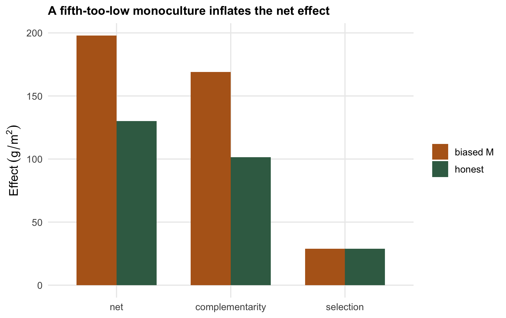
With honest references the net effect is `r sprintf("%.1f", part_true["dY"])` g/m^2^. Measure the monocultures a fifth too low and the same mixture data return a net effect of `r sprintf("%.1f", part_bias["dY"])`, an inflation of `r sprintf("%.0f", infl)`%, all of it landing in the complementarity effect; the selection effect is unchanged. Nothing about the mixture changed; only the denominator did. The check is to ask, before believing any complementarity number, whether the monocultures were grown at matched density and conditions, and to treat species that barely persist alone as a warning rather than a data point.
```{r fig-bias}
#| fig-cap: "The same mixture data, partitioned with honest monoculture references (green) and with references measured a fifth too low (ochre). Under-measured monocultures inflate the net and complementarity effects."
#| fig-alt: "Grouped bar chart of net, complementarity and selection effects; the biased-monoculture bars are much taller for net and complementarity but equal for selection."
db <- data.frame(effect = rep(c("net","complementarity","selection"), 2),
                 ref = rep(c("honest","biased M"), each = 3),
                 val = c(part_true, part_bias))
db$effect <- factor(db$effect, levels = c("net","complementarity","selection"))
ggplot(db, aes(effect, val, fill = ref)) +
  geom_col(position = "dodge", width = 0.7) +
  scale_fill_manual(values = c("honest" = col_true, "biased M" = col_bias)) +
  labs(x = NULL, y = expression(Effect~(g/m^2)), fill = NULL,
       title = "A fifth-too-low monoculture inflates the net effect")
```
## Check 2: additive or substitutive design?
A substitutive (replacement) design holds total density constant: a four-species mixture puts each species at a quarter density. An additive design adds species at full density, so the mixture is four times as dense as each monoculture. That difference alone produces more yield, and if you feed an additive experiment into the partition as if it were substitutive, the extra density is misread as a diversity effect.
```{r design}
a <- c(1.8, 2.2, 2.0, 2.4); dfull <- 100; RYe4 <- rep(1/4, 4)
mono <- a * dfull                                   # linear yield, NO interaction
sub_each <- a * (dfull / 4)                          # substitutive: quarter density each
add_each <- a * dfull                                # additive: full density each
rbind(substitutive = round(lh(mono, sub_each / mono, RYe4), 2),
      additive      = round(lh(mono, add_each / mono, RYe4), 2))
```
There is no interaction here at all: yield is a fixed multiple of density. The substitutive design correctly returns a net effect of `r sprintf("%.0f", sub_part["dY"])`. The additive design returns `r sprintf("%.0f", add_part["dY"])` g/m^2^ of pure phantom overyielding, all of it from the extra plants. The check is to know which design produced the data, and to compare a mixture only with monocultures at the matching total density.
Even substitutive designs raise a quieter question when yield does not rise in proportion to density. When the yield-density curve saturates, a species grown at a quarter density that meets no competition from the other species returns more than a quarter of its full-density monoculture, and the partition reports complementarity. In the saturating case here, with still no interaction between species, the net effect comes out at `r sprintf("%.1f", sat_sub["dY"])` g/m^2^; whether that counts as complementarity or as an artefact of the curve is part of the debate noted at the end of this post.
## Check 3: is one species running the selection effect?
The selection effect is a covariance, and a covariance can be set by a single extreme point. If one species has a far larger monoculture yield than the rest, its term in the sum can swamp everyone else's.
```{r dominant}
Mc   <- c(90, 140, 180, 220, 900); RYe5 <- rep(1/5, 5)
dRYc <- c(0.14, 0.10, 0.06, 0.02, 0.20)
part_c <- lh(Mc, RYe5 + dRYc, RYe5)
cross  <- (dRYc - mean(dRYc)) * (Mc - mean(Mc))     # per-species contribution to selection
round(rbind(partition = part_c), 2)
round(cross, 2)
```
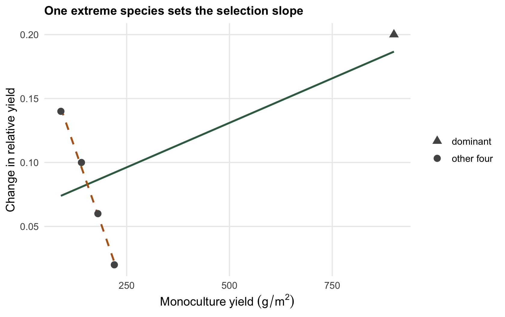
The selection effect is `r sprintf("%.1f", part_c["sel"])` g/m^2^ and looks positive: the productive species overperform. But one species (monoculture yield `r max(Mc)`) supplies `r sprintf("%.0f", sp5_share)`% of it. Among the other four, the relationship between monoculture yield and relative-yield change is the opposite sign, so removing that one species turns the selection contribution to `r sprintf("%.1f", sel_drop)`, a reversal. A selection effect that flips when you drop a single species is a description of that species, not of the community.
```{r fig-dominant}
#| fig-cap: "Selection as a covariance. Fitted across all five species (green) the slope is positive; drop the one extreme species and the line through the other four (ochre) tilts the other way. One species sets the sign."
#| fig-alt: "Scatter of relative-yield change against monoculture yield; a green line through all five points slopes upward, an ochre line through the four non-extreme points slopes downward."
dc <- data.frame(M = Mc, dRY = dRYc, grp = c(rep("other four",4), "dominant"))
ggplot(dc, aes(M, dRY)) +
  geom_smooth(data = dc, method = "lm", se = FALSE, colour = col_true, linewidth = 0.9) +
  geom_smooth(data = subset(dc, grp == "other four"), method = "lm", se = FALSE,
              colour = col_bias, linewidth = 0.9, linetype = "dashed") +
  geom_point(aes(shape = grp), size = 3, colour = col_ref) +
  scale_shape_manual(values = c("dominant" = 17, "other four" = 16)) +
  labs(x = expression(Monoculture~yield~(g/m^2)), y = "Change in relative yield",
       shape = NULL, title = "One extreme species sets the selection slope")
```
## The honest limit
These checks bound a biodiversity-ecosystem function result; they do not validate the biology. A partition can survive all three, with matched monocultures, a clean substitutive design, and no single dominant species, and still only describe a pattern. It says the mixture used the site more completely than expected and tells you whether the gain was spread evenly or concentrated in the productive species. It does not tell you the mechanism, and its own interpretation is still debated (Hooper et al. 2005 Ecological Monographs 75(1):3-35; Pillai and Gouhier 2019 Ecology 100(7):e02645). A net effect that is corroborated only by the partition is a weaker claim than one backed by a measured process. Run the checks, report both effects, and keep the mechanism as a separate question.
## References
- Fox JW 2005. Ecology Letters 8(8):846-856 (10.1111/j.1461-0248.2005.00795.x).
- Hooper DU et al. 2005. Ecological Monographs 75(1):3-35 (10.1890/04-0922).
- Loreau M 1998. Oikos 82(3):600-602 (10.2307/3546381).
- Loreau M, Hector A 2001. Nature 412(6842):72-76 (10.1038/35083573).
- Pillai P, Gouhier TC 2019. Ecology 100(7):e02645 (10.1002/ecy.2645).
## Related tutorials
- [Complementarity and selection effects](../complementarity-and-selection-effects/)
- [Partitioning the net biodiversity effect](../partitioning-the-net-biodiversity-effect/)
- [Biodiversity and ecosystem function in R](../biodiversity-and-ecosystem-function/)
- [Ecosystem multifunctionality and its threshold](../multifunctionality-and-the-threshold/)