---
title: "Partitioning the net biodiversity effect"
description: "The Loreau-Hector additive partition in R from scratch: split the net biodiversity effect into complementarity and selection, and see the identity hold."
date: "2026-06-29 12:00"
date-modified: "2026-10-01"
categories: [ecology tutorial, R, biodiversity, ecosystem function, community ecology]
image: thumbnail.png
image-alt: "A single stacked bar splitting the net biodiversity effect into a complementarity part and a selection part."
---
*Corrected 1 October 2026: the post said that Loreau and Hector's erratum fixed a formula slip, although it redrew figure panels whose regression lines were faint or missing; it now says so, and the title of the decomposition figure no longer claims that the four mixtures share one net effect.*
*Corrected 30 September 2026: the post said the two extreme mixtures give the same net effect, although their printed net effects differ; it now says both are overyielding mixtures whose partitions describe opposite ecologies.*
```{r setup}
#| code-fold: true
#| code-summary: "Setup: packages, colours and plot theme"
#| results: hide
#| message: false
#| warning: false
knitr::opts_chunk$set(echo = TRUE, message = FALSE, warning = FALSE,
                      dev = "png", dpi = 120, fig.path = "figures/",
                      fig.width = 7, fig.height = 4.4)
library(ggplot2)
theme_te <- theme_minimal(base_size = 12) +
  theme(panel.background = element_rect(fill = "#f5f4ee", colour = NA),
        plot.background  = element_rect(fill = "#f5f4ee", colour = NA),
        panel.grid.minor = element_blank(),
        plot.title = element_text(face = "bold", size = 12))
theme_set(theme_te)
col_comp <- "#3a6b52"; col_sel <- "#b5651d"; col_ref <- "#555555"

## Loreau-Hector partition, population covariance so the identity is exact
lh <- function(M, RYo, RYe) {
  dRY <- RYo - RYe; N <- length(M)
  dY   <- sum(dRY * M)
  comp <- N * mean(dRY) * mean(M)
  sel  <- N * mean((dRY - mean(dRY)) * (M - mean(M)))
  c(dY = dY, comp = comp, sel = sel, resid = dY - comp - sel)
}

set.seed(387)
M   <- round(runif(6, 80, 700))
RYe <- rep(1/6, 6)
both  <- lh(M, RYe + (0.05 + 0.00040 * (M - mean(M))), RYe)
pcomp <- lh(M, RYe + 0.08, RYe)
psel  <- lh(M, RYe + 0.0005 * (M - mean(M)), RYe)
negs  <- lh(M, RYe + (0.09 - 0.00030 * (M - mean(M))), RYe)
max_resid <- max(abs(c(both["resid"], pcomp["resid"], psel["resid"], negs["resid"])))

## scatter data for the 'both' mixture
dRY_both <- (0.05 + 0.00040 * (M - mean(M)))
scat <- data.frame(M = M, dRY = dRY_both)
```
The [previous post](../biodiversity-and-ecosystem-function/) measured the net biodiversity effect: how much more a mixture yields than the sum of its species' sown shares of their monocultures. A positive net effect is a fact, but it is not an explanation. The mixture might overyield because the species partition resources and each does a little better than expected, or because one productive species takes over and pulls the average up. Those are different biology, and the standard tool for separating them is the additive partition of Loreau and Hector 2001 Nature 412(6842):72-76.
The partition splits the net effect into two named pieces, a **complementarity effect** and a **selection effect**, and the split is an exact algebraic identity, not an approximation. This post derives it, codes it from scratch, and shows what each piece means.
## The identity
Write the net effect as a sum over the `r length(M)` species in the mixture. For species *i*, let `M[i]` be its monoculture yield, `RYe[i]` its expected relative yield (its sown fraction) and `RYo[i]` its observed relative yield in the mixture. Let the deviation be `dRY[i] = RYo[i] - RYe[i]`. Then the net effect is
$$\Delta Y = \sum_i \Delta RY_i \, M_i .$$
Multiply and divide by the number of species *N*. The sum becomes *N* times the mean of the products, and the mean of a product is the product of means plus their covariance:
$$\Delta Y = N \, \overline{\Delta RY \cdot M} = N\,\overline{\Delta RY}\;\overline{M} \; + \; N\,\text{cov}(\Delta RY, M).$$
The first term is the complementarity effect, the second is the selection effect. The covariance here divides by *N*, not by *N* minus one; that is what makes the two pieces add back to the net effect exactly.
```{r partition-fn}
lh <- function(M, RYo, RYe) {
  dRY <- RYo - RYe; N <- length(M)
  dY   <- sum(dRY * M)
  comp <- N * mean(dRY) * mean(M)               # complementarity
  sel  <- N * mean((dRY - mean(dRY)) * (M - mean(M)))  # selection (population cov)
  c(dY = dY, comp = comp, sel = sel, resid = dY - comp - sel)
}
```
## One mixture
Take six species with the monoculture yields below, sown in equal sixths, and give them relative yields that rise gently with monoculture yield, so both pieces are non-zero.
```{r one-mixture}
set.seed(387)
M   <- round(runif(6, 80, 700))
RYe <- rep(1/6, 6)
RYo <- RYe + (0.05 + 0.00040 * (M - mean(M)))
round(lh(M, RYo, RYe), 4)
```
The net effect is `r sprintf("%.1f", both["dY"])` g/m^2^. Of that, `r sprintf("%.1f", both["comp"])` is complementarity and `r sprintf("%.1f", both["sel"])` is selection, and the residual is exactly zero: the two pieces reconstruct the net effect to machine precision. Across all four example mixtures below the largest residual is zero up to floating-point rounding: a rounding error, not a model error. The partition is arithmetic.
```{r fp-guard-1}
#| include: false
stopifnot(max_resid / max(abs(c(both["dY"], pcomp["dY"], psel["dY"], negs["dY"]))) < 1e-10)
```
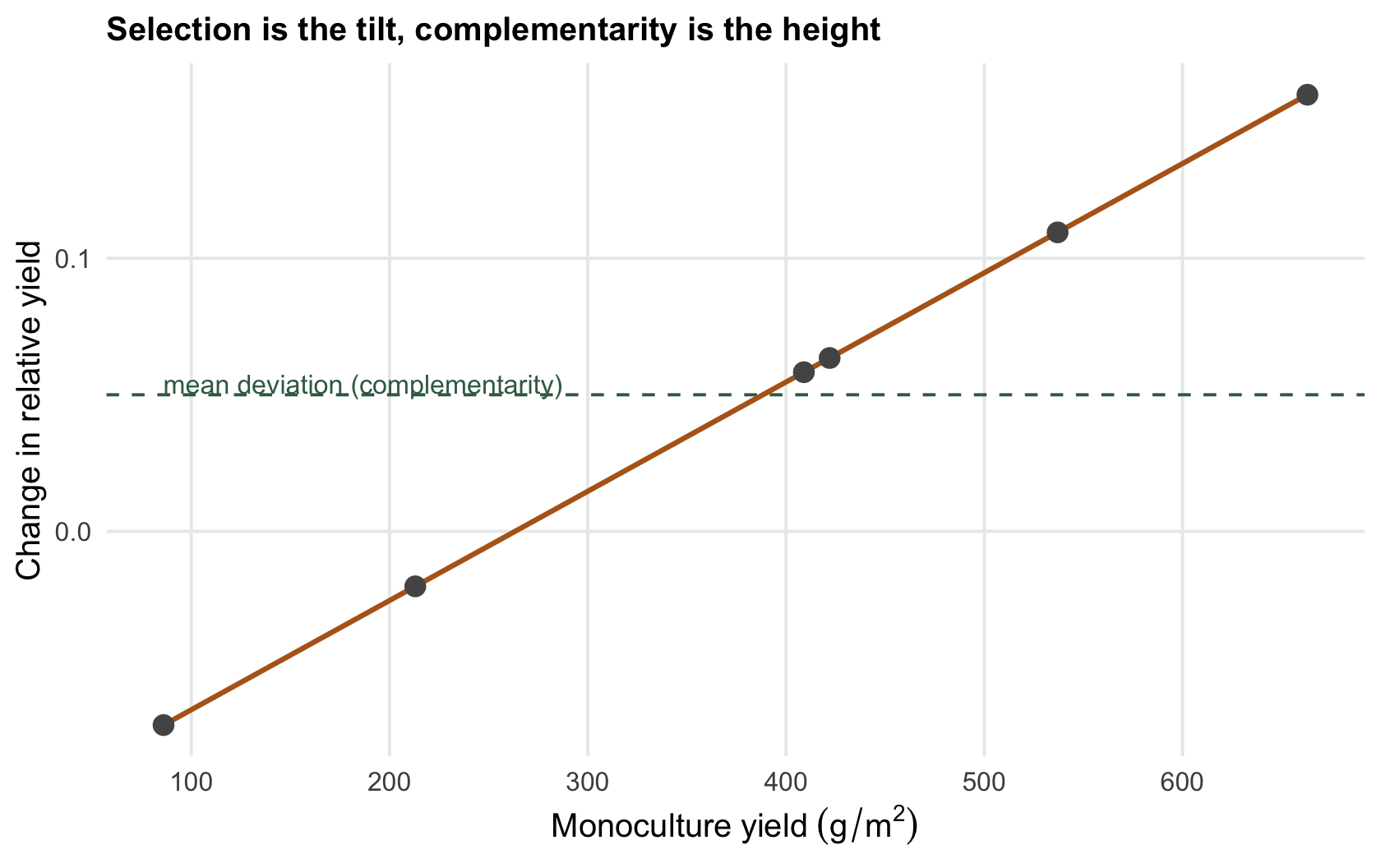
The complementarity effect is *N* times the average deviation in relative yield, scaled by the average monoculture. It answers: on average, do the species do better in the mixture than their sown share predicts? The selection effect is *N* times the covariance between monoculture yield and the deviation in relative yield. It answers a different question: are the deviations concentrated in the productive species? A positive selection effect means the high-monoculture species are the ones overperforming.
```{r fig-scatter}
#| fig-cap: "The selection effect is a covariance. Change in relative yield plotted against monoculture yield for the six species; the upward tilt (the covariance) is the selection effect, the average height is the complementarity per unit."
#| fig-alt: "Scatter of change in relative yield against monoculture yield for six species, with a rising fitted line indicating a positive covariance."
ggplot(scat, aes(M, dRY)) +
  geom_hline(yintercept = mean(scat$dRY), colour = col_comp, linetype = "dashed") +
  geom_smooth(method = "lm", se = FALSE, colour = col_sel, linewidth = 0.9) +
  geom_point(size = 3, colour = col_ref) +
  annotate("text", x = min(M), y = mean(scat$dRY) + 0.004,
           label = "mean deviation (complementarity)", colour = col_comp, hjust = 0, vjust = -0.4, size = 3.4) +
  labs(x = expression(Monoculture~yield~(g/m^2)),
       y = "Change in relative yield",
       title = "Selection is the tilt, complementarity is the height")
```
## The two extremes, and a warning
Because the pieces are independent, a positive net effect can be built entirely from one or the other. If every species has the same deviation in relative yield, the covariance with monoculture yield is zero, so the whole net effect is complementarity. If the average deviation is zero but the productive species overperform, the whole net effect is selection.
```{r extremes}
pcomp <- lh(M, RYe + 0.08, RYe)                     # constant deviation
psel  <- lh(M, RYe + 0.0005 * (M - mean(M)), RYe)   # zero-mean, correlated with M
rbind(pure_complementarity = round(pcomp, 2), pure_selection = round(psel, 2))
```
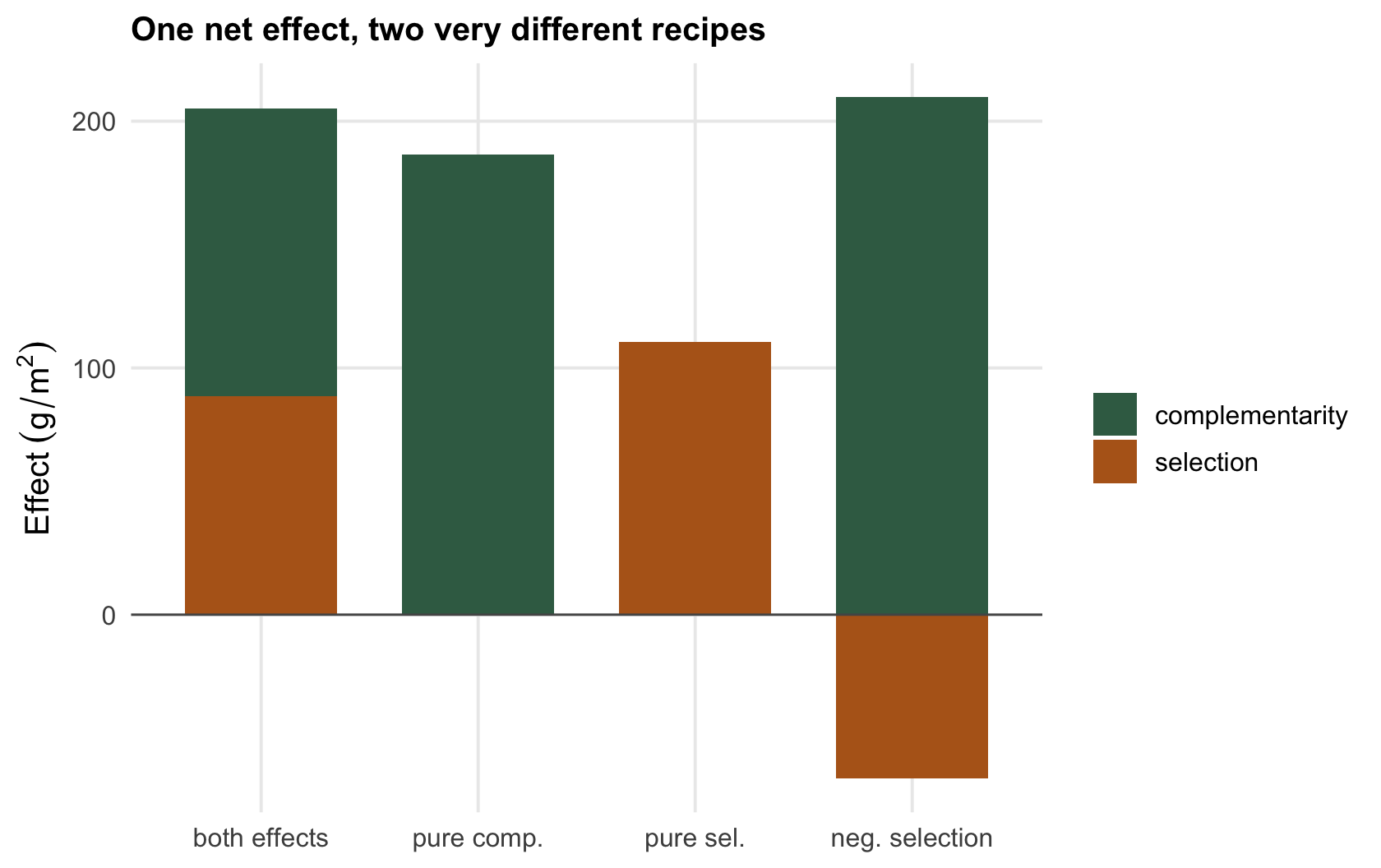
The pure-complementarity mixture has a net effect of `r sprintf("%.1f", pcomp["dY"])`, all of it complementarity, with a selection effect of `r sprintf("%.1f", pcomp["sel"])`. The pure-selection mixture has a net effect of `r sprintf("%.1f", psel["dY"])`, all of it selection. Read only the net effect and both are simply overyielding mixtures; read the partition and they are opposite ecologies.
There is a subtler case worth building, because it is where the partition earns its keep. A mixture can have a positive net effect *and a negative selection effect*: the productive species gain least, and the subordinate species carry the mixture.
```{r negative-selection}
negs <- lh(M, RYe + (0.09 - 0.00030 * (M - mean(M))), RYe)
round(negs, 2)
```
Here the net effect is `r sprintf("%.1f", negs["dY"])`, but complementarity is `r sprintf("%.1f", negs["comp"])` while selection is `r sprintf("%.1f", negs["sel"])`. The complementarity is larger than the net effect, and selection drags it back down: every species beats its sown share here, but the small ones beat it by far more than the big ones. A single net number would hide all of that.
```{r fig-decomp}
#| fig-cap: "The net biodiversity effect of four mixtures split into complementarity (green) and selection (ochre). The last mixture has a positive net effect despite a negative selection effect: its ochre part sits below zero, so its net effect is the green height less the ochre depth, not the top of its bar."
#| fig-alt: "Stacked bar chart of four mixtures, each split into a green complementarity part and an ochre selection part; the fourth bar has a selection part below zero."
dec <- data.frame(
  mix  = rep(c("both effects","pure comp.","pure sel.","neg. selection"), each = 2),
  part = rep(c("complementarity","selection"), 4),
  val  = c(both["comp"], both["sel"], pcomp["comp"], pcomp["sel"],
           psel["comp"], psel["sel"], negs["comp"], negs["sel"]))
dec$mix <- factor(dec$mix, levels = c("both effects","pure comp.","pure sel.","neg. selection"))
ggplot(dec, aes(mix, val, fill = part)) +
  geom_col(width = 0.7) +
  geom_hline(yintercept = 0, colour = col_ref, linewidth = 0.4) +
  scale_fill_manual(values = c(complementarity = col_comp, selection = col_sel)) +
  labs(x = NULL, y = expression(Effect~(g/m^2)), fill = NULL,
       title = "Two ingredients, very different recipes")
```
## What the partition does not settle
The partition is exact and it is worth running on every biodiversity experiment, but it names *patterns*, not *mechanisms*. A large complementarity effect is consistent with resource partitioning, with facilitation, and with a mixture escaping a shared pest; the number cannot tell you which. The selection effect is a covariance, with all the fragility that implies, and it can be dominated by one extreme species. Loreau and Hector's own erratum (Nature 413:548) concerns the figures, not the partition: it redrew panels of the original whose regression lines were faint or missing. Fox 2005 Ecology Letters 8(8):846-856 later split the selection effect further, into a dominance effect and a trait-dependent complementarity effect.
The next post takes the interpretation seriously: why the selection effect is a covariance rather than a mechanism, and what you can and cannot read off these two numbers.
## References
- Cardinale BJ et al. 2007. Proceedings of the National Academy of Sciences 104(46):18123-18128 (10.1073/pnas.0709069104).
- Fox JW 2005. Ecology Letters 8(8):846-856 (10.1111/j.1461-0248.2005.00795.x).
- Loreau M 1998. Oikos 82(3):600-602 (10.2307/3546381).
- Loreau M, Hector A 2001. Nature 412(6842):72-76 (10.1038/35083573); erratum Nature 413:548 (10.1038/35097128).
## Related tutorials
- [Biodiversity and ecosystem function in R](../biodiversity-and-ecosystem-function/)
- [Complementarity and selection effects](../complementarity-and-selection-effects/)
- [Ecosystem multifunctionality and its threshold](../multifunctionality-and-the-threshold/)
- [Checking a biodiversity-function analysis](../checking-a-biodiversity-ecosystem-function-analysis/)