---
title: "Multilevel selection and group structure"
description: "Split the Price equation into between-group and within-group terms in R, and build a case where cooperators lose inside every group yet rise in the population."
date: "2026-07-09 10:00"
date-modified: "2026-10-14"
categories: [evolutionary ecology, evolutionary game theory, R, ecology tutorial]
image: thumbnail.png
image-alt: "Three panels of before and after bars: the cooperator fraction falls inside both groups while the population-wide fraction rises"
---
*Corrected 14 October 2026: the post said small groups make the condition harder to meet; it now says they need a wider spread between groups but a smaller excess over random assortment than large groups.*
*Corrected 7 October 2026: the post said variance in group composition is relatedness by another name and that the between-group and within-group terms map onto the benefit and cost terms of the kin selection account; it now says relatedness measures the excess of that variance over random assortment and that the two accounts do not match term by term. It also said reshuffling into random groups destroys between-group variance, where it returns that variance to the random-assortment level.*
The Price equation splits change in a trait into a selection term and a transmission term. It can be split a second time. If the population is divided into groups, the covariance between fitness and trait value can be written as a covariance between group means plus an average of the covariances inside groups. That is the law of total covariance, applied to evolution, and it gives an exact accounting identity:
$$\bar{w}\,\Delta \bar{z} = \operatorname{Cov}_g\!\left(\bar{w}_g, \bar{z}_g\right) + \mathbb{E}_g\!\left(\bar{w}_g \Delta \bar{z}_g\right)$$
The first term is between-group selection: groups with more cooperators do better as groups. The second is within-group selection: inside any one group, cooperators do worse than the defectors they subsidise. The two terms have opposite signs for a cooperative trait, and the outcome is whichever wins.
This post builds a population where the within-group term is negative in every single group and the population-wide cooperator frequency rises anyway. That is Simpson's paradox with an evolutionary payload, and it is the honest core of what multilevel selection means.
## A group-structured population
Each group has `m` members. A cooperator pays a cost `c` and delivers a benefit `b` split equally among the other `m - 1` members of its group, so it receives nothing from its own act. With `k` cooperators in a group, a cooperator collects benefits from the other `k - 1` cooperators and a defector collects from all `k`.
```{r}
#| label: population
pcov <- function(x, y) mean(x * y) - mean(x) * mean(y)   # population covariance

make_pop <- function(kvec, m, b, cost, w0 = 1) {
  do.call(rbind, lapply(seq_along(kvec), function(g) {
    k <- kvec[g]
    z   <- c(rep(1, k), rep(0, m - k))                   # 1 = cooperator
    pay <- ifelse(z == 1, -cost + b * (k - 1) / (m - 1), b * k / (m - 1))
    data.frame(group = g, z = z, w = w0 + pay)
  }))
}

pop <- make_pop(kvec = c(2, 8), m = 10, b = 5, cost = 1)
print(aggregate(cbind(z, w) ~ group, pop, mean))
```
Two groups of ten, one with two cooperators and one with eight. The cooperator-rich group has a mean fitness of `r round(mean(pop$w[pop$group == 2]), 1)` against `r round(mean(pop$w[pop$group == 1]), 1)`, which is where the between-group term will come from. The group mean payoff works out to exactly `(b - c)` times the cooperator fraction, so a group's productivity is linear in how cooperative it is.
Inside each group the picture is the reverse.
```{r}
#| label: within
for (g in 1:2) {
  d  <- subset(pop, group == g)
  wc <- mean(d$w[d$z == 1]); wd <- mean(d$w[d$z == 0])
  cat(sprintf("group %d: x = %.2f   cooperator %.4f   defector %.4f   difference %+.6f\n",
              g, mean(d$z), wc, wd, wc - wd))
}
cat("algebra says the difference is -c - b/(m-1) =", -1 - 5 / 9, "\n")
```
Defectors out-earn cooperators by the same amount in both groups, and that amount does not depend on the group's composition at all. A cooperator forgoes `c` and hands `b/(m-1)` to each other member, including the defector it is being compared with, so the gap is `c + b/(m-1)` regardless of `k`. Within-group selection against cooperation is constant here, which makes the accounting unusually clean.
## The partition
```{r}
#| label: price
price_parts <- function(pop) {
  gm <- aggregate(cbind(z, w) ~ group, pop, mean)
  list(between = pcov(gm$w, gm$z),
       within  = mean(sapply(split(pop, pop$group), function(d) pcov(d$w, d$z))),
       total   = pcov(pop$w, pop$z),
       wbar    = mean(pop$w),
       zbar    = mean(pop$z))
}

p <- price_parts(pop)
cat(sprintf("between %+.6f   within %+.6f   total %+.6f\n", p$between, p$within, p$total))
cat("identity holds:", all.equal(p$total, p$between + p$within), "\n")
cat(sprintf("mean fitness %.4f   change in cooperator frequency %+.6f\n",
            p$wbar, p$total / p$wbar))
cat(sprintf("cooperator frequency: %.6f before, %.6f after\n",
            p$zbar, p$zbar + p$total / p$wbar))
```
Between-group selection contributes `r round(p$between, 2)` and within-group selection contributes `r sprintf("%.4f", p$within)`, so the total is positive and the cooperator frequency rises from 0.5 to `r sprintf("%.4f", p$zbar + p$total / p$wbar)`. The identity is checked with `all.equal` rather than asserted, which matters: an identity that has been rearranged by hand is exactly the kind of thing that survives a plausibility check and fails a numeric one.
## The paradox made explicit
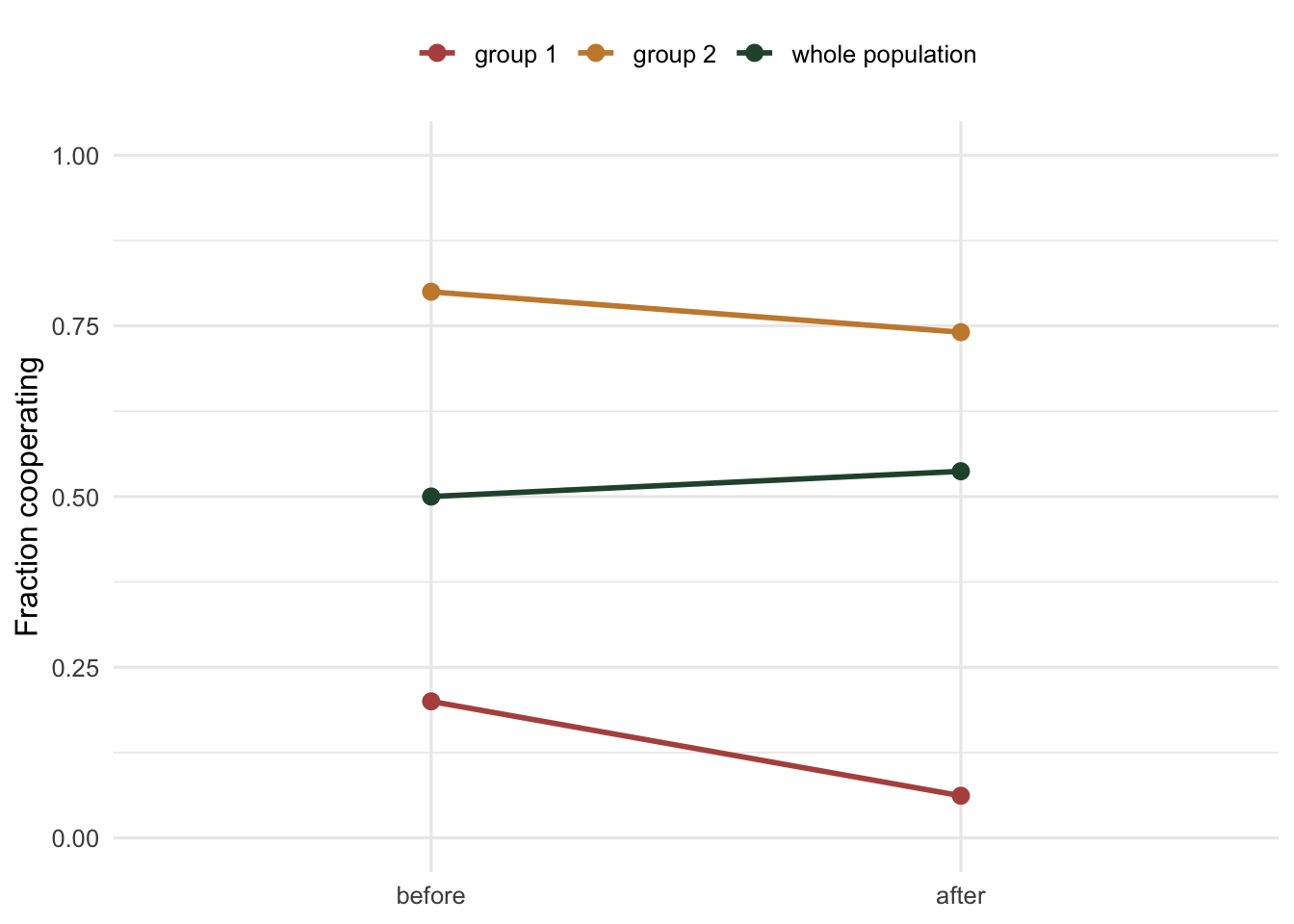
Track the cooperator fraction inside each group as well as across the population.
```{r}
#| label: fig-simpson
#| fig-cap: "Cooperator fraction before and after one round of selection. Inside both groups the fraction falls; across the population it rises, because the cooperator-rich group contributes more than twice as many offspring."
#| fig-alt: "Three pairs of connected points: two group lines sloping downwards and a population line sloping upwards."
library(ggplot2)
te_canvas <- theme(plot.background  = element_rect(fill = "#f5f4ee", colour = NA),
                   panel.background = element_rect(fill = "#f5f4ee", colour = NA))
after_group <- sapply(1:2, function(g) {
  d <- subset(pop, group == g)
  mean(d$z) * mean(d$w[d$z == 1]) / mean(d$w)
})
before_group <- sapply(1:2, function(g) mean(subset(pop, group == g)$z))
d <- data.frame(
  level = factor(rep(c("group 1", "group 2", "whole population"), each = 2),
                 levels = c("group 1", "group 2", "whole population")),
  time  = rep(c("before", "after"), 3),
  x     = c(before_group[1], after_group[1], before_group[2], after_group[2],
            p$zbar, p$zbar + p$total / p$wbar))
d$time <- factor(d$time, levels = c("before", "after"))
cat(sprintf("group 1: %.6f -> %.6f\ngroup 2: %.6f -> %.6f\nwhole:   %.6f -> %.6f\n",
            d$x[1], d$x[2], d$x[3], d$x[4], d$x[5], d$x[6]))
ggplot(d, aes(time, x, group = level, colour = level)) +
  geom_line(linewidth = 1) +
  geom_point(size = 2.6) +
  scale_colour_manual(values = c(`group 1` = "#b5534e", `group 2` = "#c98a3a",
                                 `whole population` = "#275139")) +
  ylim(0, 1) +
  labs(x = NULL, y = "Fraction cooperating", colour = NULL) +
  theme_minimal(base_size = 12) + te_canvas + theme(legend.position = "top")
```
Group 1 goes from 0.2 to `r sprintf("%.4f", after_group[1])` and group 2 from 0.8 to `r sprintf("%.4f", after_group[2])`. Both fall. The population goes from 0.5 to `r sprintf("%.4f", p$zbar + p$total / p$wbar)`. Nothing has been smuggled in: group 2 simply produces more than twice the offspring of group 1, so the population-wide average shifts towards group 2's composition faster than either group's composition erodes.
This is why "cooperators do worse than defectors" and "cooperation is increasing" can both be true statements about the same population at the same moment. Whether they are depends entirely on how much of the trait variance sits between groups rather than within them.
## Where the sign flips
Because both terms have closed forms in this model, the condition can be located exactly instead of scanned. Between-group selection is `(b - c)` times the variance in group composition, and within-group selection is `-(c + b/(m-1))` times the average within-group variance.
```{r}
#| label: closedform
gm <- aggregate(cbind(z, w) ~ group, pop, mean)
cat("between equals (b - c) Var(x):",
    all.equal(p$between, (5 - 1) * pcov(gm$z, gm$z)), "\n")
cat("within equals -(c + b/(m-1)) E[x(1-x)]:",
    all.equal(p$within, -(1 + 5 / 9) * mean(gm$z * (1 - gm$z))), "\n")
```
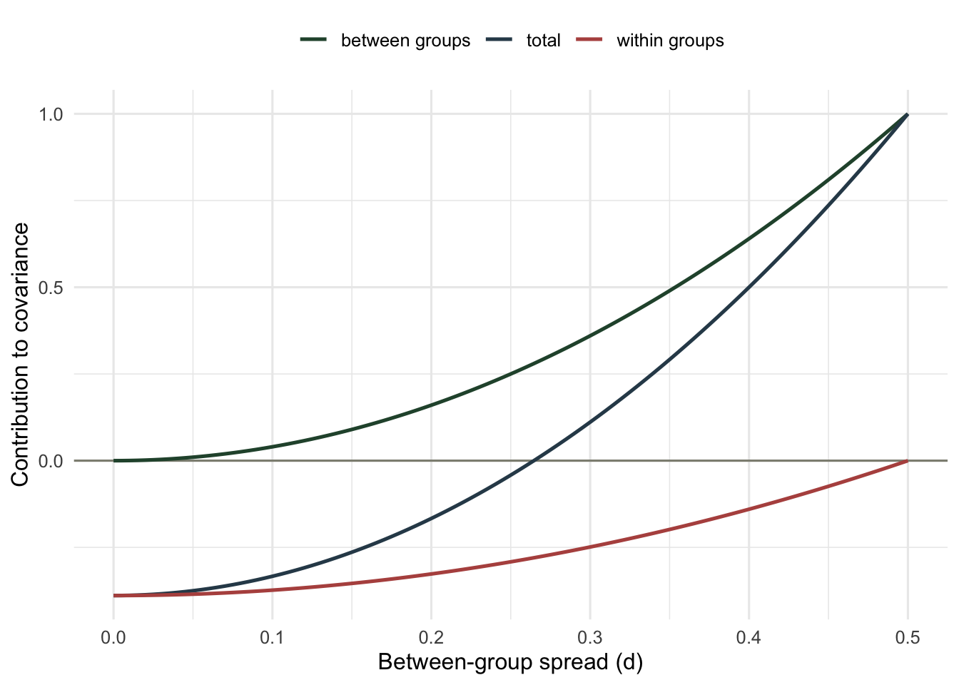
Now put two groups at `0.5 - d` and `0.5 + d` and increase the spread.
```{r}
#| label: fig-spread
#| fig-cap: "The two components of change against between-group spread, for two groups of ten with b = 5 and c = 1. Between-group selection grows as the square of the spread while within-group selection weakens, and the total crosses zero near a spread of 0.265."
#| fig-alt: "A rising curve for the between-group term, a shallow rising negative curve for the within-group term, and their sum crossing zero at about 0.265."
components <- function(d, m = 10, b = 5, cost = 1) {
  x   <- c(0.5 - d, 0.5 + d)
  bet <- (b - cost) * pcov(x, x)
  wit <- -(cost + b / (m - 1)) * mean(x * (1 - x))
  c(between = bet, within = wit, total = bet + wit)
}
ds <- seq(0, 0.5, by = 0.005)
cm <- as.data.frame(t(sapply(ds, components)))
cm$d <- ds
print(round(cm[cm$d %in% c(0, 0.1, 0.25, 0.3, 0.4, 0.5), c("d", "between", "within", "total")], 5),
      row.names = FALSE)
long <- data.frame(d = rep(ds, 3), value = c(cm$between, cm$within, cm$total),
                   term = rep(c("between groups", "within groups", "total"), each = length(ds)))
ggplot(long, aes(d, value, colour = term)) +
  geom_hline(yintercept = 0, colour = "#8d8d80") +
  geom_line(linewidth = 0.9) +
  scale_colour_manual(values = c(`between groups` = "#275139",
                                 `within groups` = "#b5534e", total = "#2f4858")) +
  labs(x = "Between-group spread (d)", y = "Contribution to covariance", colour = NULL) +
  theme_minimal(base_size = 12) + te_canvas + theme(legend.position = "top")
```
The crossing point has a closed form. Setting the two terms equal gives a required spread of half the square root of `q / ((b - c) + q)`, where `q` is the within-group penalty `c + b/(m-1)`.
```{r}
#| label: threshold
q     <- 1 + 5 / 9
root  <- uniroot(function(d) components(d)["total"], c(0.01, 0.49), tol = 1e-12)$root
exact <- 0.5 * sqrt(q / (4 + q))
cat(sprintf("numeric root %.8f   closed form %.8f\n", root, exact))
cat("agree:", all.equal(root, exact, tolerance = 1e-6), "\n")
for (m in c(2, 4, 10, 25, 100, 1000)) {
  qm <- 1 + 5 / (m - 1)
  cat(sprintf("m = %4d   within-group penalty %.4f   spread needed %.6f\n",
              m, qm, 0.5 * sqrt(qm / (4 + qm))))
}
cat("limit for very large groups:", format(0.5 * sqrt(1 / 5), digits = 8), "\n")
```
Small groups need a wider spread, not a narrower one, in this parameterisation. In a group of two the cooperator's entire benefit lands on the single partner it is competing with, so the within-group penalty is `c + b`, and the required spread is `r sprintf("%.3f", 0.5 * sqrt((1 + 5 / (2 - 1)) / (4 + 1 + 5 / (2 - 1))))`. In very large groups the benefit is diluted across many members, the penalty falls to `c` alone, and the required spread drops towards `r sprintf("%.4f", 0.5 * sqrt(1 / 5))`. Both limits fall out of the same expression, and neither had to be guessed.
A wider spread is not the same as a harder condition, though, because group size and group variance are not independent. Groups formed at random already differ more from one another when they are small, so the excess over random assortment that the condition needs, the yardstick the next section uses, is smaller in small groups, not larger. How far real groups exceed that random level is the part this calculation cannot supply. Small groups formed by siblings will have high between-group variance for genetic reasons, and that is where the group and kin accounts meet.
## Does it work with many groups?
The identity is not special to two groups. Draw forty groups with compositions spread across the whole range and check both the partition and the closed form.
```{r}
#| label: many
set.seed(11)
kv   <- sample(0:10, 40, replace = TRUE)
pop2 <- make_pop(kv, m = 10, b = 5, cost = 1)
p2   <- price_parts(pop2)
gm2  <- aggregate(cbind(z, w) ~ group, pop2, mean)
formula_total <- 4 * pcov(gm2$z, gm2$z) - (1 + 5 / 9) * mean(gm2$z * (1 - gm2$z))
cat(sprintf("total from data %.8f   from the formula %.8f\n", p2$total, formula_total))
cat("agree:", all.equal(p2$total, formula_total), "\n")
cat(sprintf("variance in group composition %.6f   change in frequency %+.6f\n",
            pcov(gm2$z, gm2$z), p2$total / p2$wbar))
kb <- rbinom(40, 10, 0.5)                      # individuals assorting at random
pb <- price_parts(make_pop(kb, m = 10, b = 5, cost = 1))
cat(sprintf("random assortment: variance %.6f   total %+.6f\n",
            pcov(kb / 10, kb / 10), pb$total))
many <- replicate(2000, { x <- rbinom(40, 10, 0.5) / 10
  4 * pcov(x, x) - (1 + 5 / 9) * mean(x * (1 - x)) })
cat(sprintf("positive in %d of 2000 random-assortment draws; largest %+.3f\n",
            sum(many > 0), max(many)))
```
The total comes out positive, but read what produced it before reading it as a result. `sample(0:10)` draws a group's composition uniformly, so groups run from all-defector to all-cooperator and the variance in composition is `r sprintf("%.3f", pcov(gm2$z, gm2$z))`. That is assortment, not the absence of it. Individuals dropped into groups of ten at random give a binomial spread with an expected variance of `r 0.5 * (1 - 0.5) / 10`, about a quarter as much, and the second draw above lands at `r sprintf("%.3f", pcov(kb / 10, kb / 10))` with a total of `r sprintf("%.3f", pb$total)`. Over 2000 such draws the total is negative every time, with the largest value reaching only `r sprintf("%.3f", max(many))`. Between-group selection does not come free from sampling noise at this group size, and a claim that a real system has group selection has to show the composition variance beats random assortment, not merely that it is above zero.
## An honest limit
The partition is an accounting identity, not a mechanism. Every group-structured population can be described this way, whether or not anything biologically interesting is happening, and the same change can be re-described with a different partition and different-looking terms. Choosing the group boundaries chooses the answer. That is not a flaw in the algebra; it is a reason the algebra cannot settle arguments on its own.
The same change also has a kin selection description, though not a term-by-term copy of this one. Relatedness between group mates corresponds to the variance in group composition in excess of what random assortment produces, not to the variance itself, and the kin account splits the same total into a benefit term `rb` and a cost term `-c` that do not line up with the between-group and within-group terms: under random assortment relatedness averages about zero, yet the between-group term is still positive. When people describe multilevel selection and kin selection as rival theories they usually mean two accounting schemes for one process, and the empirical questions (how much variance, at what scale, with what benefit structure) are identical under both.
Finally, this model does one round of selection on fixed groups. Nothing here forms groups, disperses offspring, or lets group composition regenerate, and those steps are where real models earn or lose their conclusions. A population that reshuffles into random groups every generation brings the between-group variance back to the random-assortment level each time, wiping out any excess as fast as selection builds it.
## References
Price GR 1970. Nature 227(5257):520-521 (10.1038/227520a0)
Wilson DS 1975. Proceedings of the National Academy of Sciences 72(1):143-146 (10.1073/pnas.72.1.143)
Traulsen A, Nowak MA 2006. Proceedings of the National Academy of Sciences 103(29):10952-10955 (10.1073/pnas.0602530103)
Nowak MA 2006. Science 314(5805):1560-1563 (10.1126/science.1133755)
## Related tutorials
- [The Price equation](../the-price-equation/)
- [Hamilton's rule and kin selection](../hamiltons-rule-and-kin-selection/)
- [Checking a kin selection analysis](../checking-a-kin-selection-analysis/)
- [F-statistics and population structure](../f-statistics-and-population-structure/)