Relatedness as a regression

evolutionary ecology
social evolution
quantitative genetics
R
ecology tutorial
What genetic relatedness really means in R: not a pedigree fraction but a regression of one genotype on another, and why the reference population matters.
Author

Tidy Ecology

Published

2026-08-06

Everyone knows full siblings are related by one half and cousins by one eighth. Fewer people know what that number actually is. In Hamilton’s rule relatedness is not a fraction of shared pedigree; it is a regression coefficient, the slope of a recipient’s genotype on an actor’s (Grafen 1985). This post estimates relatedness that way in base R, recovers the familiar pedigree values, and shows why the same pair of animals can have different relatedness depending on who you compare them against.

Relatedness is a slope

The regression definition is direct: take many pairs of social partners, regress the second partner’s breeding value on the first, and the slope is the relatedness. Simulate groups whose members share genes to a set degree, then estimate r without ever consulting a pedigree.

make_pairs <- function(r, G, p = 0.5) {
  s <- sqrt(r); founder <- rbinom(G, 1, p)
  g <- t(sapply(founder, function(f) ifelse(runif(2) < s, f, rbinom(2, 1, p))))
  g
}
set.seed(441)
estimate_r <- function(r, G = 60000) {
  g <- make_pairs(r, G)
  coef(lm(g[, 2] ~ g[, 1]))[2]                # slope = relatedness
}
for (r in c(0.5, 0.25, 0.125))
  cat(sprintf("pedigree r = %.3f  ->  estimated regression r = %.3f\n", r, estimate_r(r)))
pedigree r = 0.500  ->  estimated regression r = 0.497
pedigree r = 0.250  ->  estimated regression r = 0.250
pedigree r = 0.125  ->  estimated regression r = 0.122

The regression recovers the pedigree values: 0.497 for full sibs, 0.250 for half sibs, 0.122 for cousins, all within sampling error of the textbook fractions. Nothing here needed a family tree. Relatedness is an observable statistical association between genotypes, which is exactly why it can be estimated from genetic markers in wild populations where pedigrees are unknown (Queller and Goodnight 1989).

library(ggplot2)
set.seed(11)
g <- make_pairs(0.5, 1500)
d <- data.frame(focal = g[, 1], mate = g[, 2])
ggplot(d, aes(focal, mate)) +
  geom_jitter(width = 0.06, height = 0.06, colour = "#275139", alpha = 0.25, size = 1) +
  geom_smooth(method = "lm", se = FALSE, colour = "#b5534e", linewidth = 0.9) +
  labs(x = "Focal genotype", y = "Groupmate genotype") +
  theme_minimal(base_size = 12)
`geom_smooth()` using formula = 'y ~ x'
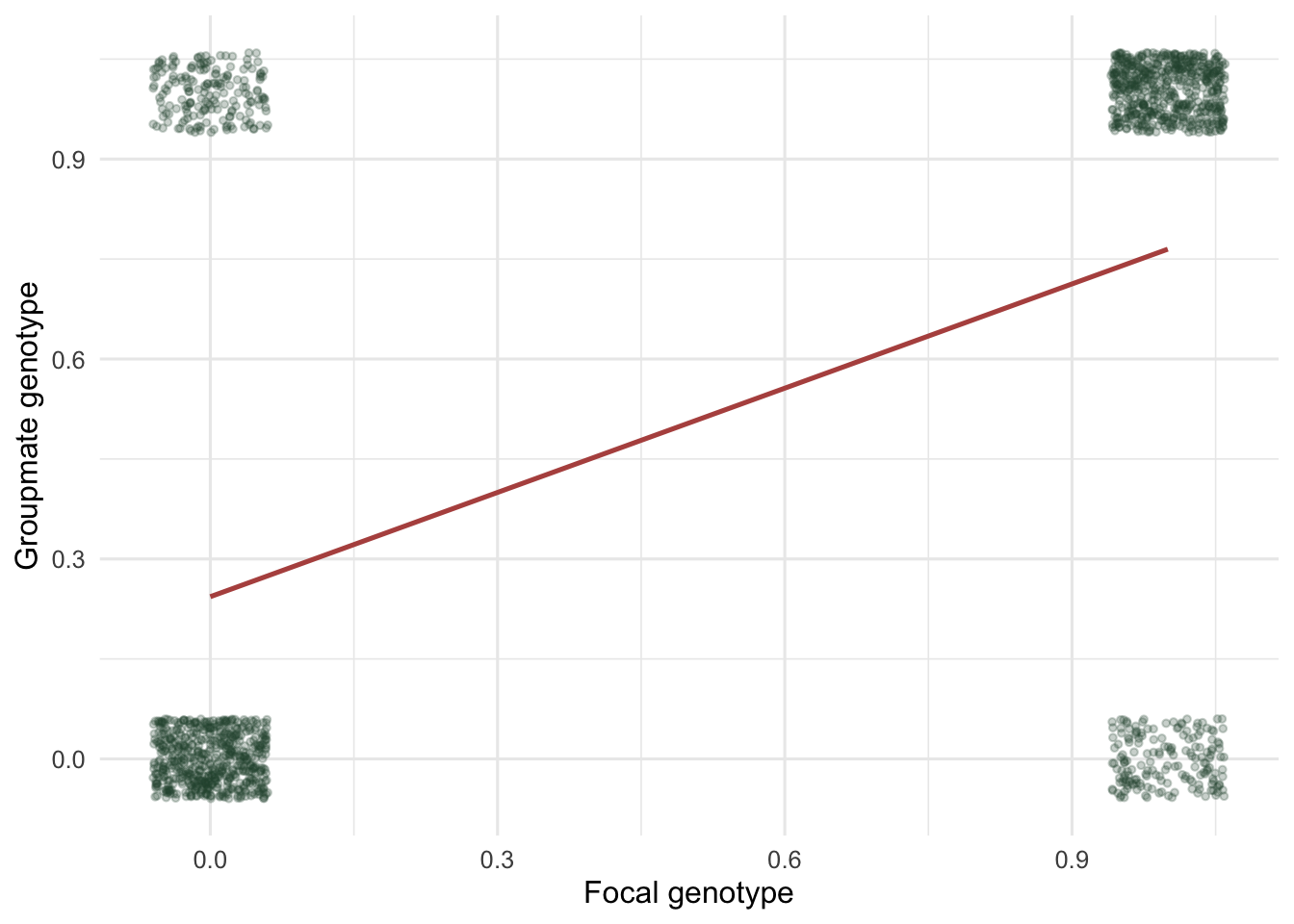
A jittered scatter of binary groupmate genotype on binary focal genotype with a green regression line of slope near one half.
Figure 1: Groupmate genotype against focal genotype for full-sibling groups. The slope of the fitted line is the relatedness, here close to 0.5; relatedness is the regression, not a pedigree fraction.

Why the reference population matters

A regression is always relative to a mean, and for relatedness that mean is the population you measure deviations from. This is not a technicality: it decides the number. Two animals that share half their genes relative to their local group can be almost unrelated relative to the whole species, if the local group is already inbred, or highly related relative to a diverse global pool. The r in Hamilton’s rule is the relatedness among the individuals who actually interact and compete, measured against the population they are drawn from, not an absolute biological constant.

This is where a common confusion starts. In a small, viscous population everyone is somewhat related in absolute terms, which seems to predict rampant altruism. But if those same relatives are also each other’s competitors, the relevant relatedness against the competitive neighbourhood can be near zero, and altruism gains nothing. Getting the reference wrong is one of the main ways a kin selection analysis goes astray, which the checking post takes up directly.

An honest limit

The regression estimate is only as good as the sample of pairs and the marker set behind the genotypes, and it inherits the usual regression frailties: rare alleles give noisy slopes, and population structure that you have not accounted for inflates apparent relatedness between individuals who merely come from similar backgrounds. That last point is the same shared-ancestry problem that drives phylogenetic regression: correlated genotypes can reflect common descent rather than the local kinship the model intends. Relatedness is a clean idea and a slippery measurement, and the slipperiness is all about choosing the right comparison.
References

Grafen A 1985. A geometric view of relatedness. Oxford Surveys in Evolutionary Biology 2:28-89

Queller DC, Goodnight KF 1989. Evolution 43(2):258-275 (10.1111/j.1558-5646.1989.tb04226.x)

Hamilton WD 1964. Journal of Theoretical Biology 7(1):1-16 (10.1016/0022-5193(64)90038-4)

Newsletter

Get new tutorials by email

New R and QGIS tutorials for ecologists, straight to your inbox. No spam; unsubscribe anytime.

By subscribing you agree to receive these emails and confirm your address once. See the privacy policy.