The hawk-dove game and the ESS

Model animal conflict in R with the hawk-dove game: the mixed evolutionarily stable strategy, the invasion criterion, and replicator dynamics converging to it.

When two animals contest a resource, the best move depends on what everyone else is doing. Escalate against a peaceful rival and you win; escalate against another fighter and you both get hurt. There is no single best strategy, only a best strategy given the population. This is what evolutionary game theory formalises, and the hawk-dove game of Maynard Smith and Price (1973) is its founding example. This post builds the game in base R, finds its evolutionarily stable strategy, and watches replicator dynamics settle onto it.

The game

Two contestants meet over a resource worth V. A hawk always escalates; a dove displays and retreats if the other escalates. Hawk against dove: the hawk takes V, the dove gets nothing. Dove against dove: they share, V/2 each. Hawk against hawk: they fight, and the loser pays an injury cost C, so each expects (V - C) / 2. The interesting case is V < C: fighting costs more than the prize.

V <- 2; C <- 5
hawk_pay <- function(p) p * ((V - C) / 2) + (1 - p) * V   # payoff to a hawk when hawks are at frequency p
dove_pay <- function(p) p * 0 + (1 - p) * (V / 2)
pstar <- V / C
cat(sprintf("mixed ESS: fraction of hawks p* = V/C = %.3f\n", pstar))

mixed ESS: fraction of hawks p* = V/C = 0.400

cat(sprintf("at p*, hawk payoff = %.3f, dove payoff = %.3f\n", hawk_pay(pstar), dove_pay(pstar)))

at p*, hawk payoff = 0.600, dove payoff = 0.600

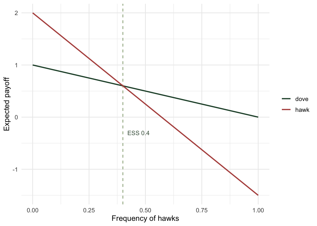
At a hawk frequency of V/C = 0.4, hawks and doves earn exactly the same, 0.6. That equality is the signature of a mixed evolutionarily stable strategy: when neither type does better, neither can spread, and the population sits still.

The invasion criterion

An ESS is a strategy that, once common, cannot be invaded by any rare alternative. The test is direct: compare the payoffs away from p*.

cat(sprintf("hawks rare (p=0.2): hawk %.3f vs dove %.3f -> hawks do better\n", hawk_pay(0.2), dove_pay(0.2)))

hawks rare (p=0.2): hawk 1.300 vs dove 0.800 -> hawks do better

cat(sprintf("hawks common (p=0.6): hawk %.3f vs dove %.3f -> doves do better\n", hawk_pay(0.6), dove_pay(0.6)))

hawks common (p=0.6): hawk -0.100 vs dove 0.400 -> doves do better

When hawks are rare they mostly meet doves and win easily, so they invade. When hawks are common they mostly meet each other and pay the injury cost (the hawk payoff even goes negative, -0.1), so doves invade instead. Each type is favoured when rare: this is negative frequency-dependent selection, the same balancing force that lets a rare strategy hold its place. Neither pure hawk nor pure dove is stable; only the 0.4 mix is.

Dynamics: getting there

The invasion argument says the mix is stable, but does a population actually reach it? The replicator equation answers this by letting each strategy grow in proportion to how far its payoff beats the population average.

replicate_hd <- function(p0, dt = 0.01, tmax = 60) {
  p <- p0; trace <- numeric(tmax / dt)
  for (i in seq_along(trace)) {
    wbar <- p * hawk_pay(p) + (1 - p) * dove_pay(p)
    p <- p + dt * p * (hawk_pay(p) - wbar)
    trace[i] <- p
  }
  trace
}
tr <- replicate_hd(0.05)
cat(sprintf("starting from 5%% hawks, the population converges to %.3f (ESS = %.3f)\n",
            tail(tr, 1), pstar))

starting from 5% hawks, the population converges to 0.400 (ESS = 0.400)

From almost all doves, hawks spread until they hit 0.4 and then stop. The ESS is not just uninvadable; here it is also an attractor, the resting point the dynamics find on their own.

library(ggplot2)
p <- seq(0, 1, 0.01)
d <- rbind(data.frame(p = p, pay = hawk_pay(p), type = "hawk"),
           data.frame(p = p, pay = dove_pay(p), type = "dove"))
ggplot(d, aes(p, pay, colour = type)) +
  geom_vline(xintercept = pstar, linetype = "dashed", colour = "#93a87f") +
  geom_line(linewidth = 0.9) +
  scale_colour_manual(values = c(hawk = "#b5534e", dove = "#275139")) +
  annotate("text", x = pstar + 0.02, y = -0.3, label = "ESS 0.4", colour = "#46604a", size = 3.4, hjust = 0) +
  labs(x = "Frequency of hawks", y = "Expected payoff", colour = NULL) +
  theme_minimal(base_size = 12)

Figure 1: Payoffs to hawks and doves as the hawk frequency changes. They cross at the ESS (0.4): below it hawks win and spread, above it doves win, so the mix is stable.

An honest limit

The whole prediction rests on the numbers V and C, and those are assumed, not measured. The ESS is V/C exactly, so halving the injury cost moves the stable mix from 0.4 to something quite different, and in real animals the payoff of a fight is hard to put on the same scale as the value of the resource. The game also treats every contest as symmetric and anonymous; real disputes turn on who arrived first, who is larger, and who owns the territory, which changes the stable strategy entirely. The hawk-dove game explains why mixed populations of bold and cautious individuals persist; turning it into a quantitative forecast for a particular species needs payoffs that field data rarely provide. The checking post works through this and the trouble with finite populations.

Related tutorials

• The replicator equation
• Sex ratio evolution and the ESS
• Evolutionary games in finite populations
• Rare species advantage and coexistence

References

Maynard Smith J, Price GR 1973. Nature 246(5427):15-18 (10.1038/246015a0)

Maynard Smith J 1982. Evolution and the Theory of Games. Cambridge University Press. ISBN 978-0521288842

Hofbauer J, Sigmund K 2003. Bulletin of the American Mathematical Society 40(4):479-519 (10.1090/S0273-0979-03-00988-1)