payA <- function(i, N, M) (M[1, 1] * (i - 1) + M[1, 2] * (N - i)) / (N - 1)
payB <- function(i, N, M) (M[2, 1] * i + M[2, 2] * (N - i - 1)) / (N - 1)

rho_game <- function(M, N, w, focal = "A") {
  if (focal == "B") M <- M[2:1, 2:1]
  g <- sapply(1:(N - 1), function(i) {
    fa <- 1 - w + w * payA(i, N, M)
    fb <- 1 - w + w * payB(i, N, M)
    fb / fa
  })
  1 / (1 + sum(cumprod(g)))
}

game <- function(a, b, c, d) {
  matrix(c(a, b, c, d), 2, 2, byrow = TRUE,
         dimnames = list(c("A", "B"), c("A", "B")))
}

# interior equilibrium of the replicator dynamics, the invasion barrier
xstar <- function(M) (M[2, 2] - M[1, 2]) / (M[1, 1] - M[1, 2] - M[2, 1] + M[2, 2])Evolutionary games in finite populations
evolutionary ecology
evolutionary game theory
natural selection
R
ecology tutorial
Evolutionary game theory in a finite population with base R: frequency-dependent fitness, exact fixation probabilities, the one-third law and risk dominance.
Corrected 27 September 2026: this post said the N = 100 sweep puts the one-third crossing away from exactly one third; the sweep brackets it between 0.30 and 0.35, which contains one third, so it shows no such offset.
The replicator equation assumes an infinite, well-mixed population. Real populations are finite, and finiteness does more than add noise: it changes which strategy wins. A strategy that the replicator equation calls unbeatable can still be replaced, and a strategy that starts below its own invasion barrier can still take over, because drift carries a few copies uphill often enough to matter.
This post puts a two-strategy game inside the Moran process and computes the fixation probability exactly. Nothing here is simulated. The whole thing is a product of ratios, and the interesting behaviour comes out of the arithmetic.
If the birth-death machinery is unfamiliar, The Moran process and fixation probability sets it up with constant fitness first.
Fitness that depends on who else is there
Take a population of fixed size N with two strategies, A and B, and a payoff matrix
\[ \begin{pmatrix} a & b \\ c & d \end{pmatrix} \]
where a is what an A player gets against another A, b what an A gets against a B, and so on. If there are i players using A, an A player meets one of the other i - 1 A players or one of the N - i B players. Excluding self-interaction, the expected payoffs are
\[ \pi_A(i) = \frac{a(i-1) + b(N-i)}{N-1}, \qquad \pi_B(i) = \frac{ci + d(N-i-1)}{N-1} \]
Payoff is not fitness. The usual translation is a baseline of 1 plus a payoff contribution scaled by an intensity of selection w:
\[ f_A(i) = 1 - w + w\,\pi_A(i) \]
with w between 0 and 1. At w = 0 everything is neutral; at w = 1 fitness is payoff. Small w is called weak selection, and most of the analytical results live there.
The Moran process now runs exactly as before, except the transition probabilities use these frequency-dependent fitnesses. The fixation probability of a single A in a population of B has a closed form:
\[ \rho_A = \frac{1}{1 + \sum_{k=1}^{N-1} \prod_{i=1}^{k} \gamma_i}, \qquad \gamma_i = \frac{f_B(i)}{f_A(i)} \]
That is the whole calculation. Each gamma_i says how much harder it is to gain a copy of A than to lose one when there are i copies around, and the cumulative products accumulate the difficulty.
Swapping the rows and columns of the matrix turns the A calculation into the B calculation, so one function covers both directions.
Two bistable games
Both games below are coordination games: A beats A, B beats B, and the replicator equation has an unstable interior point x*. Above x* the A frequency rises to one, below it falls to zero. x* is the invasion barrier that A must clear.
G1 <- game(5, 1, 2, 2)
G2 <- game(4, 1, 3, 2)
N <- 100
w <- 0.01

for (nm in c("G1", "G2")) {
  M <- get(nm)
  ra <- rho_game(M, N, w)
  rb <- rho_game(M, N, w, "B")
  cat(sprintf("%s  x*=%.4f  rhoA=%.6f (%.3f x 1/N)  rhoB=%.6f (%.3f x 1/N)  rhoA/rhoB=%.3f\n",
              nm, xstar(M), ra, ra * N, rb, rb * N, ra / rb))
}
G1 x*=0.2500 rhoA=0.011166 (1.117 x 1/N) rhoB=0.004321 (0.432 x 1/N) rhoA/rhoB=2.584
G2 x*=0.5000 rhoA=0.008393 (0.839 x 1/N) rhoB=0.008588 (0.859 x 1/N) rhoA/rhoB=0.977In the infinite population both games say the same thing: a single A player is below the barrier and goes extinct. In the finite population they say different things. In G1, with a barrier at one quarter, a single A fixes with probability 0.011166, which is 1.117 times the neutral value of 1/N. Selection is helping A, even though A starts far below its own barrier. In G2, with a barrier at one half, a single A fixes with probability 0.008393, which is 0.839 times neutral. There selection is working against A.
The ratio of the two directions tells a related but distinct story. In G1, A is 2.584 times as likely to replace B as B is to replace A. In G2 the ratio is 0.977, marginally the other way.
Where the asymmetry comes from
The whole result sits in gamma_i, the per-step handicap. Plotting it against the A frequency shows the barrier directly.
suppressMessages(library(ggplot2))
te_canvas <- theme(plot.background  = element_rect(fill = "#f5f4ee", colour = NA),
                   panel.background = element_rect(fill = "#f5f4ee", colour = NA))

gam <- function(M, N, w) {
  i <- 1:(N - 1)
  (1 - w + w * payB(i, N, M)) / (1 - w + w * payA(i, N, M))
}

dr <- rbind(
  data.frame(x = (1:99) / 100, g = gam(G1, 100, 0.01), game = "G1, barrier at 0.25"),
  data.frame(x = (1:99) / 100, g = gam(G2, 100, 0.01), game = "G2, barrier at 0.50"))

ggplot(dr, aes(x, g, colour = game)) +
  geom_hline(yintercept = 1, colour = "#8d8d80", linewidth = 0.6) +
  geom_line(linewidth = 1.1) +
  scale_colour_manual(values = c("G1, barrier at 0.25" = "#275139",
                                 "G2, barrier at 0.50" = "#b5534e")) +
  labs(x = "Frequency of A", y = expression(f[B] / f[A]), colour = NULL) +
  theme_minimal(base_size = 12) + te_canvas +
  theme(legend.position = "top", panel.grid.minor = element_blank())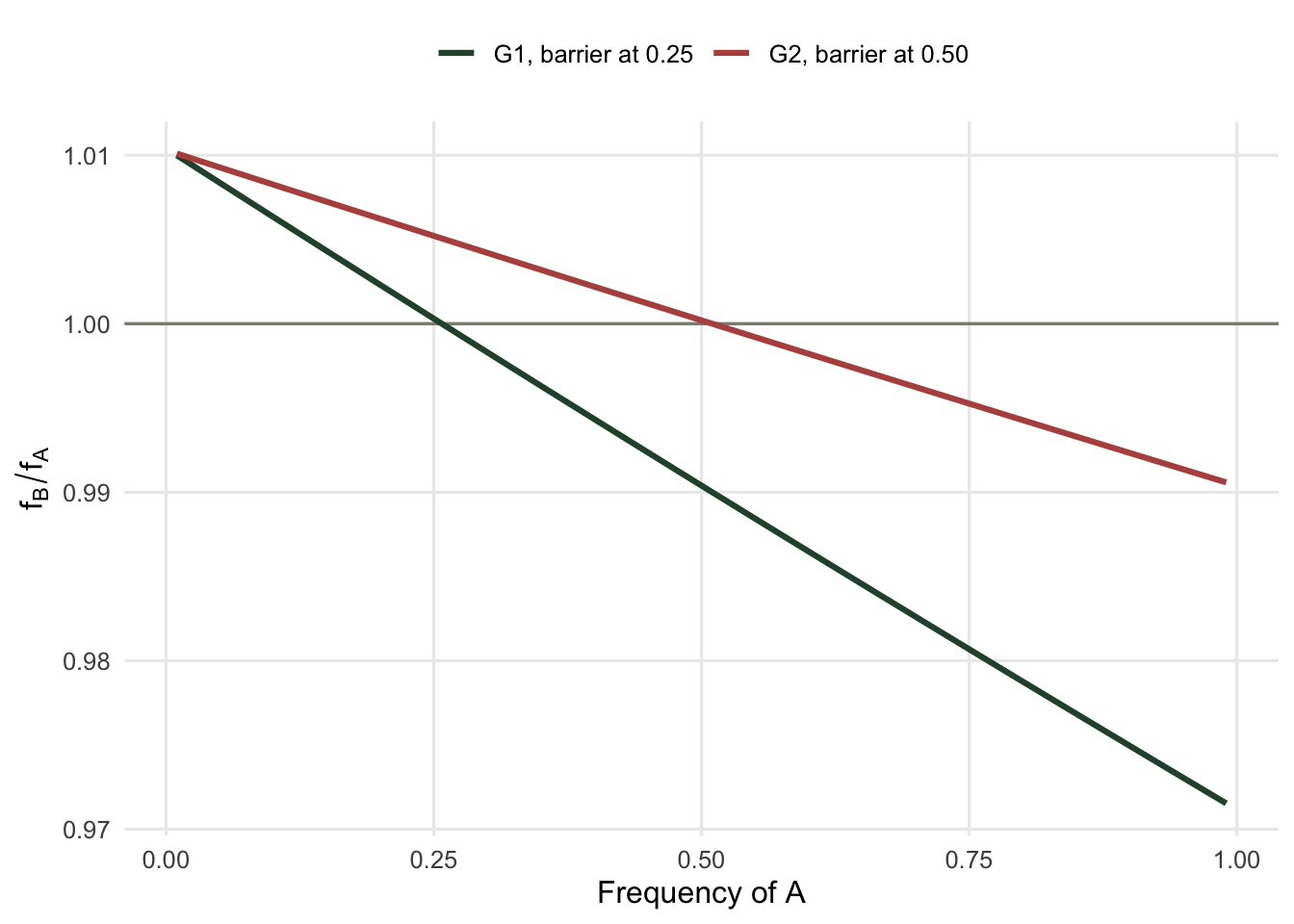
Both curves start above one, so a lone A is fighting the current in both games. The difference is how long the fight lasts. In G1 the curve drops below one near a quarter, so the run of unfavourable steps is short and the products stay small. In G2 the unfavourable stretch covers half the axis, and the products blow up. Fixation probability is not set by whether the first step is favourable; it is set by the whole accumulated path.
The crossings sit slightly to the right of the replicator barriers. That offset is the self-exclusion correction: an A player interacts with N - 1 others rather than with the population as a whole, so a rare A meets fewer A players than the frequency alone would suggest. The offset shrinks as N grows.
Two different questions, two different thresholds
There are two natural ways to ask whether selection favours A, and they are not the same question.
The first compares rho_A to 1/N, the neutral value. This asks whether a mutant A does better than a strategically irrelevant mutant would. The second compares rho_A to rho_B, which asks which direction the population flips more readily over long stretches of time. Sweeping the invasion barrier separates them.
# a one-parameter family of bistable games with barrier at xs
mk <- function(xs) game(2, 0, 3 - 1 / xs, 1)

d <- data.frame(xstar = seq(0.15, 0.65, by = 0.05))
d$A_over_1N <- sapply(d$xstar, function(x) rho_game(mk(x), 100, 0.002) * 100)
d$A_over_B <- sapply(d$xstar, function(x)
  rho_game(mk(x), 100, 0.002) / rho_game(mk(x), 100, 0.002, "B"))
print(round(d, 4), row.names = FALSE)
xstar A_over_1N A_over_B
0.15 1.1204 1.5937
0.20 1.0651 1.3479
0.25 1.0321 1.2192
0.30 1.0102 1.1404
0.35 0.9947 1.0873
0.40 0.9830 1.0491
0.45 0.9740 1.0204
0.50 0.9668 0.9979
0.55 0.9609 0.9800
0.60 0.9559 0.9652
0.65 0.9518 0.9529The first comparison crosses one between a barrier of 0.30 and 0.35. The second crosses one between 0.45 and 0.50. Those are the two classical results, both due to Nowak and colleagues in 2004. Under weak selection and large N, selection favours A over neutral drift when the barrier is below one third, and A is more likely to replace B than the reverse when the barrier is below one half, which is the risk dominance condition already familiar from economics.
xs <- seq(0.12, 0.68, by = 0.01)
dd <- rbind(
  data.frame(xstar = xs, value = sapply(xs, function(x) rho_game(mk(x), 100, 0.002) * 100),
             comparison = "rho_A against 1/N"),
  data.frame(xstar = xs, value = sapply(xs, function(x)
    rho_game(mk(x), 100, 0.002) / rho_game(mk(x), 100, 0.002, "B")),
    comparison = "rho_A against rho_B"))

ggplot(dd, aes(xstar, value, colour = comparison)) +
  geom_hline(yintercept = 1, colour = "#8d8d80", linewidth = 0.6) +
  geom_vline(xintercept = c(1 / 3, 1 / 2), colour = "#8d8d80",
             linetype = "22", linewidth = 0.6) +
  geom_line(linewidth = 1.1) +
  scale_colour_manual(values = c("rho_A against 1/N" = "#275139",
                                 "rho_A against rho_B" = "#b5534e")) +
  labs(x = "Invasion barrier of A", y = "Ratio", colour = NULL) +
  theme_minimal(base_size = 12) + te_canvas +
  theme(legend.position = "top", panel.grid.minor = element_blank())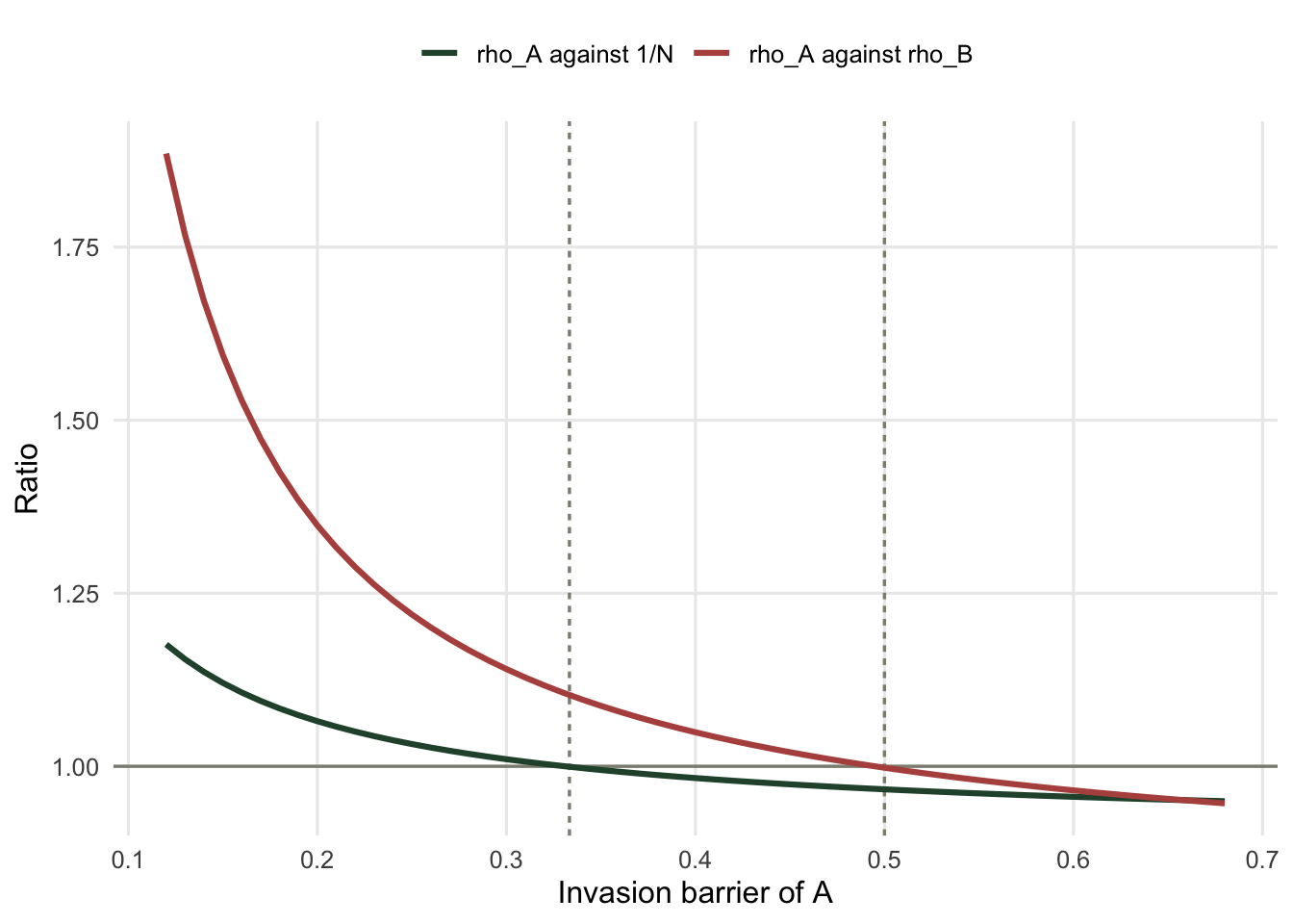
One third is a genuinely surprising number. The naive guess is one half: if A has to clear a barrier below the midpoint it should be favoured. The extra demand comes from the shape of the fixation path. A rare mutant starts at the bottom of the range, where the per-step ratio is still above one and A is losing ground, and it has to be carried across that whole unfavourable stretch before the game turns in its favour. That cost tightens the threshold rather than loosening it: the barrier has to sit below one third, not merely below one half, before A beats neutral drift.
Weak selection is about wN, not w
The one-third law is a weak-selection result, and it is easy to read “weak” as “small w”. It is not. The relevant quantity is wN.
M <- mk(0.30)
for (wn in c(0.01, 0.1, 1, 3)) {
  cat(sprintf("wN=%5.2f  ", wn))
  for (Nv in c(10, 100, 1000)) {
    cat(sprintf("N=%4d: %.5f   ", Nv, rho_game(M, Nv, wn / Nv) * Nv))
  }
  cat("\n")
}
wN= 0.01 N= 10: 1.00061 N= 100: 1.00056 N=1000: 1.00055
wN= 0.10 N= 10: 1.00587 N= 100: 1.00536 N=1000: 1.00532
wN= 1.00 N= 10: 1.03680 N= 100: 1.03246 N=1000: 1.03210
wN= 3.00 N= 10: 0.96713 N= 100: 0.98547 N=1000: 0.98666 Three population sizes spanning two orders of magnitude give almost the same answer when wN is matched. At wN = 1 the three values are 1.03680, 1.03246 and 1.03210. That means a selection intensity of 0.1 in a population of ten behaves like an intensity of 0.001 in a population of a thousand. Reporting w alone tells the reader nothing about how strong selection really was.
wn <- 10^seq(-2, log10(5), length.out = 60)
dw <- do.call(rbind, lapply(c(1000, 100, 10), function(Nv)
  data.frame(wn = wn, Nv = factor(Nv, levels = c("1000", "100", "10")),
             v = sapply(wn, function(z) rho_game(M, Nv, z / Nv) * Nv))))

cat("peak of the N = 1000 curve at wN =",
    round(wn[which.max(dw$v[dw$Nv == "1000"])], 3), "\n")
peak of the N = 1000 curve at wN = 1.271 # widest line drawn first so the coincident curves stay visible
ggplot(dw, aes(wn, v, colour = Nv, linewidth = Nv)) +
geom_hline(yintercept = 1, colour = "#8d8d80", linewidth = 0.6) +
geom_line() +
scale_x_log10() +
scale_linewidth_manual(values = c("1000" = 2.4, "100" = 1.2, "10" = 0.5)) +
scale_colour_manual(values = c("1000" = "#c8d2cc", "100" = "#93a87f",
"10" = "#275139")) +
labs(x = "wN", y = expression(rho[A] %*% N), colour = "N") +
guides(linewidth = "none",
colour = guide_legend(override.aes = list(linewidth = 1.6))) +
theme_minimal(base_size = 12) + te_canvas +
theme(legend.position = "top", panel.grid.minor = element_blank())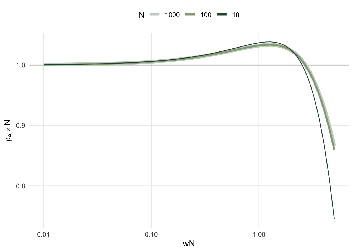
The curve peaks at wN around 1.271 and then falls back through one. Selection that is too strong is worse for A than selection that is moderate, because strong selection makes the early unfavourable steps nearly impassable. Drift is not only noise here; it is the mechanism that gets A across its barrier.
Strict Nash is not enough
In the infinite population, A is a strict Nash equilibrium whenever a > c: a lone B player among A players does worse than the residents. Finiteness weakens that. A lone B among N - 1 A players meets A players in N - 1 of its interactions, while an A player meets only N - 2 other A players and one B. The correct finite comparison is a(N-2) + b > c(N-1), which can fail even when a > c.
G4 <- game(3, 0, 2.9, 1)
c1 <- function(M, N) M[1, 1] * (N - 2) + M[1, 2] - M[2, 1] * (N - 1)
cat("G4 invasion barrier x* =", round(xstar(G4), 6), "\n")
G4 invasion barrier x* = 0.909091 for (Nv in c(5, 10, 20, 31, 32, 50, 100)) {
cat(sprintf("N=%4d c1=%+7.3f %-16s rhoB*N=%.6f %s\n", Nv, c1(G4, Nv),
if (c1(G4, Nv) > 0) "B cannot invade" else "B can invade",
rho_game(G4, Nv, 0.01, "B") * Nv,
if (rho_game(G4, Nv, 0.01, "B") * Nv < 1) "replacement opposed" else "replacement favoured"))
}N= 5 c1= -2.600 B can invade rhoB*N=1.018411 replacement favoured
N= 10 c1= -2.100 B can invade rhoB*N=1.025063 replacement favoured
N= 20 c1= -1.100 B can invade rhoB*N=1.038362 replacement favoured
N= 31 c1= +0.000 B can invade rhoB*N=1.052974 replacement favoured
N= 32 c1= +0.100 B cannot invade rhoB*N=1.054301 replacement favoured
N= 50 c1= +1.900 B cannot invade rhoB*N=1.078154 replacement favoured
N= 100 c1= +6.900 B cannot invade rhoB*N=1.143944 replacement favouredThe first condition is exactly zero at N = 31 and positive from N = 32 on, and the strict test in the code counts that exact tie as invadable. At N = 31 and below, a rare B invades a population of A players even though A is a strict Nash equilibrium of the underlying game. Small populations are structurally kinder to rare strategies.
The second condition is the more interesting failure. Nowak and colleagues define a strategy as evolutionarily stable in a finite population (ESS_N) only if both conditions hold: selection opposes a rare B invading, and selection opposes B replacing A. Here the second never holds at any size tested, because the barrier the one-third rule applies to is the invader’s own: B’s barrier is 0.091, far below one third, which is the same as saying A’s barrier of 0.909 is above two thirds. So A is a strict Nash equilibrium of the game, is uninvadable by a rare mutant for N above 31, and is still the strategy that loses over long time scales. Nash stability and long-run persistence come apart once the population is finite.
An honest limit
The exact formula assumes a great deal. Fitness is linear in payoff, which keeps f_A positive only while w is small enough that no payoff drives it negative; with the payoffs used here that constraint never binds, but it will for matrices with large negative entries. Interactions are with a uniformly drawn partner from the rest of the population, so there is no spatial structure, no assortment and no repeated interaction with the same opponent. The population size is fixed, which for the reasons set out in the Moran post is not the same as an ecologically constant population.
The most restrictive assumption is that mutation is rare enough that the population is nearly always monomorphic. The whole framework asks a single mutant lineage to reach fixation or extinction before the next one appears. With more mutation, several strategies coexist at once and the fixation probability stops being the right summary. That regime needs a different tool.
The 1/3 result is also asymptotic in N. The sweep above is at N = 100, but its steps of 0.05 bracket the crossing between 0.30 and 0.35, an interval that contains one third, so it cannot show how far a finite population moves the threshold. The companion post Checking a finite population model works through how far off the asymptotic conditions can be at sizes an ecologist would actually study.
References
Nowak, Sasaki, Taylor, Fudenberg 2004 Nature 428(6983):646-650 (10.1038/nature02414)
Taylor, Fudenberg, Sasaki, Nowak 2004 Bull Math Biol 66(6):1621-1644 (10.1016/j.bulm.2004.03.004)
Imhof, Nowak 2006 J Math Biol 52(5):667-681 (10.1007/s00285-005-0369-8)
Nowak 2006 “Evolutionary Dynamics: Exploring the Equations of Life” ISBN 978-0674023383