---
title: "Checking a finite population model"
description: "Diagnostics for finite population models in R: how many replicates a fixation probability needs, why weak selection scales with wN, and when branching is real."
date: "2026-07-10 09:00"
date-modified: "2026-10-14"
categories: [evolutionary ecology, evolutionary game theory, model diagnostics, R, ecology tutorial]
image: thumbnail.png
image-alt: "Grouped bars comparing the number of clusters counted by two different detection rules across five mutation rates"
---
*Corrected 14 October 2026: check one explained the growth in the replicate count by the inverse square of the difference alone, and it now adds that the gap between the two fixation probabilities shrinks faster than the advantage while the variance of the rarer fixation falls; check three called the invasion barrier comfortably below one third, and it now says just below; check four spoke of genuine gaps between the spikes at low mutation, and it now says there is one.*
*Corrected 1 October 2026: check one said that another seed would sometimes let the gap clear the two standard error criterion, and it now says the gap rarely clears it because the design has too few replicates; check four said the shoulders vanish at the highest mutation rates, and it now says they remain but are no longer local maxima; the alt text of the replicate figure now describes a curve that is steeper at small advantages, not a straight line.*
The three posts before this one derive results and check that the arithmetic is right. This one asks a different question: under what conditions would those results have been visible in a study that ran a simulation instead of a derivation, and where does the asymptotic theory stop describing populations of a size an ecologist would actually work with?
Four checks, each aimed at a specific way the earlier conclusions can fail in practice.
## Check 1: how many replicates a fixation probability needs
Fixation probability is a proportion, and proportions near zero are expensive to estimate. The neutral value at `N = 100` is 0.01, so a simulation study measuring whether selection favours a mutant is trying to resolve a difference between two small numbers.
```{r}
#| label: sim
rho <- function(r, N, i = 1) if (r == 1) i / N else (1 - r^-i) / (1 - r^-N)

sim_moran <- function(r, N, i0 = 1, reps = 2000, seed = 1) {
  set.seed(seed)
  fix <- 0L
  for (k in seq_len(reps)) {
    i <- i0
    while (i > 0 && i < N) {
      birth <- runif(1) < r * i / (r * i + N - i)
      die <- runif(1) < i / N
      i <- i + (birth && !die) - (!birth && die)
    }
    fix <- fix + (i == N)
  }
  fix / reps
}

for (r in c(1.1, 1.01, 1.0)) {
  p <- sim_moran(r, 100, reps = 2000, seed = 42)
  se <- sqrt(p * (1 - p) / 2000)
  cat(sprintf("r = %.2f   simulated = %.4f (se %.5f)   exact = %.6f\n",
              r, p, se, rho(r, 100)))
}
```
Two thousand replicates resolve a mutant of relative fitness 1.1 comfortably: the simulated 0.0965 sits well clear of the neutral `r rho(1, 100)`. They do not reliably resolve a relative fitness of 1.01. The simulated value of 0.0175 has a standard error of 0.00293, and the neutral run gave 0.0125 with a standard error of 0.00248, so the gap between the two estimates is of the same order as the uncertainty attached to each of them. Change the seed and that gap rarely clears the two standard error criterion used below: the design has too few replicates to resolve the difference, whichever way one run happens to come out. A study reporting "selection had no detectable effect" from this simulation would be reporting the sample size, not the biology.
The required sample size follows from the two-proportion comparison and grows fast as the advantage shrinks.
```{r}
#| label: power
need <- function(r, N = 100) {
  p1 <- rho(r, N)
  p0 <- 1 / N
  ceiling((2 * sqrt(p1 * (1 - p1)) + 2 * sqrt(p0 * (1 - p0)))^2 / (p1 - p0)^2)
}

for (r in c(1.1, 1.05, 1.02, 1.01)) {
  cat(sprintf("r = %.2f   exact rho = %.6f   replicates for a two-se gap = %d\n",
              r, rho(r, 100), need(r)))
}
```
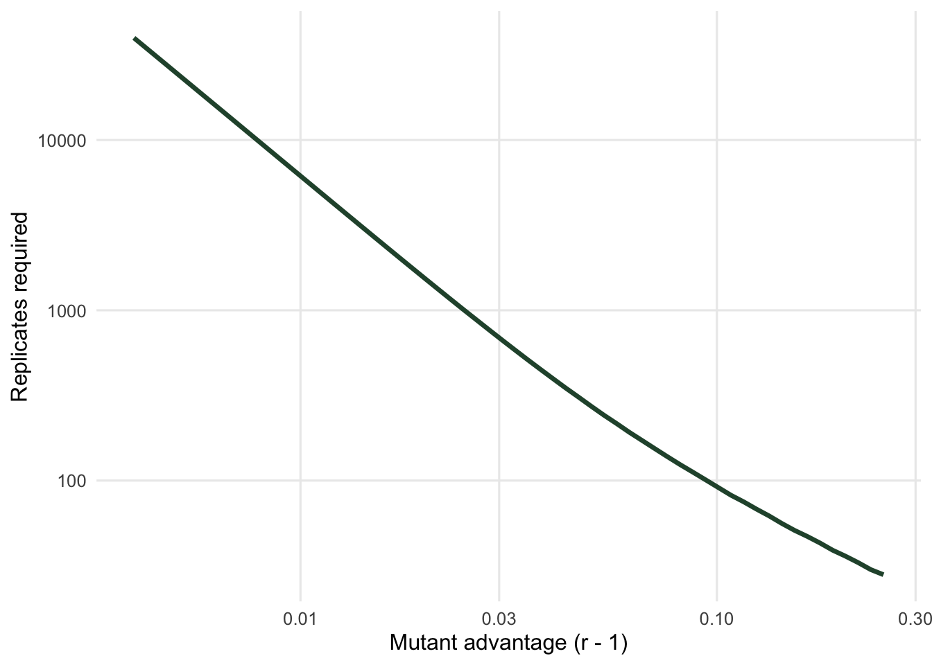
A ten per cent fitness advantage needs 92 replicates. A one per cent advantage needs 6151, a factor of 67 for a tenfold smaller effect: the required count grows with the inverse square of the difference between the two fixation probabilities, which shrinks faster than the advantage does, while the smaller variance of the rarer fixation pulls part of that growth back.
```{r}
#| label: fig-power
#| fig-cap: "Replicates needed for a two standard error separation from neutral, against the mutant advantage. Both axes are logarithmic."
#| fig-alt: "A declining curve on logarithmic axes, steeper at small advantages than at large ones, showing required replicate count falling from tens of thousands to under one hundred as the mutant advantage grows"
suppressMessages(library(ggplot2))
te_canvas <- theme(plot.background  = element_rect(fill = "#f5f4ee", colour = NA),
                   panel.background = element_rect(fill = "#f5f4ee", colour = NA))

rs <- 1 + 10^seq(-2.4, -0.6, length.out = 60)
dp <- data.frame(adv = rs - 1, n = sapply(rs, need))

ggplot(dp, aes(adv, n)) +
  geom_line(colour = "#275139", linewidth = 1.2) +
  scale_x_log10(expand = expansion(mult = c(0.02, 0.06))) +
  scale_y_log10() +
  labs(x = "Mutant advantage (r - 1)", y = "Replicates required") +
  theme_minimal(base_size = 12) + te_canvas +
  theme(panel.grid.minor = element_blank())
```
The practical reading is that the fixation probability of a weakly selected mutant is not a quantity worth simulating. The exact formula is one line and costs nothing. Simulation is for the cases where no exact formula exists, and even then the replicate count should be worked out before the run rather than after.
## Check 2: weak selection is about wN, not w
The one-third law and every other weak-selection result assume `w` is small. The mistake is to check that assumption against 1 rather than against `1/N`.
```{r}
#| label: setup-game
payA <- function(i, N, M) (M[1, 1] * (i - 1) + M[1, 2] * (N - i)) / (N - 1)
payB <- function(i, N, M) (M[2, 1] * i + M[2, 2] * (N - i - 1)) / (N - 1)

rho_game <- function(M, N, w, focal = "A") {
  if (focal == "B") M <- M[2:1, 2:1]
  g <- sapply(1:(N - 1), function(i) {
    (1 - w + w * payB(i, N, M)) / (1 - w + w * payA(i, N, M))
  })
  1 / (1 + sum(cumprod(g)))
}

game <- function(a, b, c, d) {
  matrix(c(a, b, c, d), 2, 2, byrow = TRUE,
         dimnames = list(c("A", "B"), c("A", "B")))
}
mk <- function(xs) game(2, 0, 3 - 1 / xs, 1)
```
Take a game whose invasion barrier is 0.30, below one third, so the asymptotic theory says selection favours A.
```{r}
#| label: wn
M <- mk(0.30)
for (Nv in c(10, 100, 1000)) {
  for (w in c(1e-4, 1e-3, 1e-2, 1e-1)) {
    v <- rho_game(M, Nv, w) * Nv
    cat(sprintf("N = %5d   w = %.0e   wN = %7.3f   rhoA*N = %.5f   %s\n",
                Nv, w, w * Nv, v, if (v > 1) "favoured" else "opposed"))
  }
}
```
At `N = 10` the prediction holds for every intensity tested, including `w = 0.1`. At `N = 1000` it fails at `w = 0.01`, where `rhoA*N` drops to `r sprintf("%.5f", rho_game(M, 1000, 1e-2) * 1000)`, and collapses to zero at `w = 0.1`. The same numerical value of `w` is weak selection in a small population and strong selection in a large one.
The failure is not subtle when it happens. It is a factor of two the wrong way, and it would show up as a clean simulation result contradicting the theory, with nothing in the output pointing at the cause. If a paper reports a selection intensity without reporting `wN`, the number cannot be interpreted.
## Check 3: the asymptotic condition against the exact one
The one-third law is a large-`N` result. The exact weak-selection condition at finite `N` is
$$
a(N-2) + b(2N-1) > c(N+1) + d(2N-4)
$$
which reduces to the one-third law only as `N` grows. For most payoff matrices the two agree at any `N` worth caring about. It is possible to construct one where they do not.
```{r}
#| label: g3
xstar <- function(M) (M[2, 2] - M[1, 2]) / (M[1, 1] - M[1, 2] - M[2, 1] + M[2, 2])
cond <- function(M, N) {
  M[1, 1] * (N - 2) + M[1, 2] * (2 * N - 1) - M[2, 1] * (N + 1) - M[2, 2] * (2 * N - 4)
}

G3 <- game(10, 0, 7.9, 1)
cat("G3 invasion barrier x* =", round(xstar(G3), 6), "(below one third)\n\n")
for (Nv in c(10, 50, 100, 200, 239, 240, 300, 1000)) {
  v <- rho_game(G3, Nv, 1e-4) * Nv
  cat(sprintf("N = %5d   condition = %+9.3f   rhoA*N = %.6f   %s\n",
              Nv, cond(G3, Nv), v, if (v > 1) "favoured" else "opposed"))
}
```
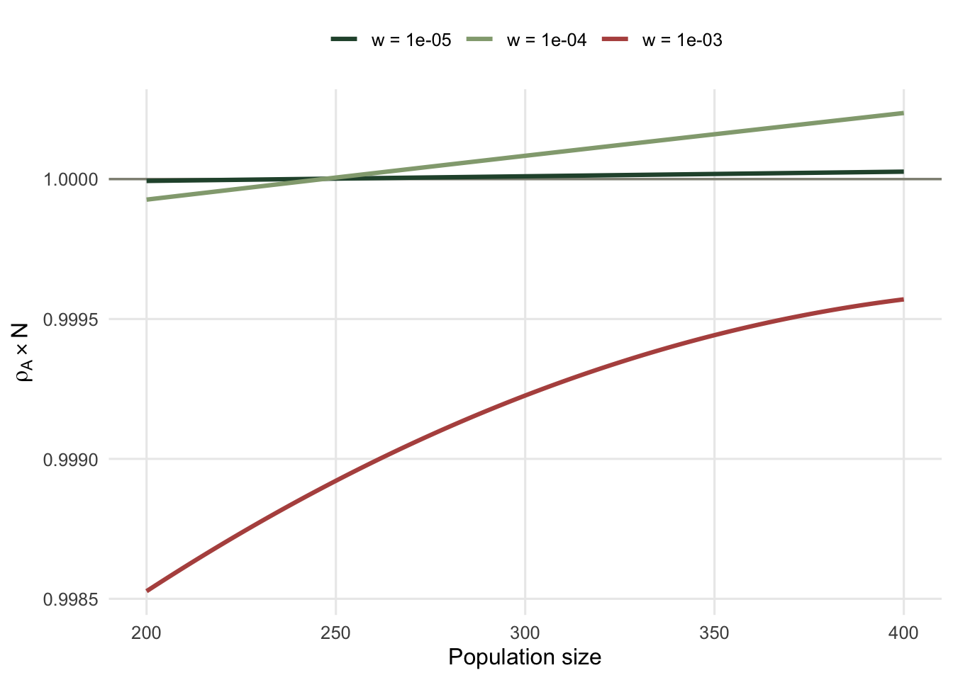
The barrier is `r round(xstar(G3), 6)`, just below one third, so the asymptotic law says A is favoured at every size. The exact linear condition disagrees for small populations: it is negative up to 238, exactly zero at 239, and positive from 240 upwards. The exact fixation probability follows the linear condition and not the asymptotic law, so in a population of a hundred this game's A strategy is opposed by selection despite satisfying the one-third criterion. The linear condition is itself a `w` approaching zero limit, so the sign change in the table sits a little above 239: at the `w = 1e-4` used here A is still opposed at 240 and only turns favoured at 247.
Where exactly the crossing sits depends on the selection intensity, which is the check-2 lesson reappearing.
```{r}
#| label: crossing
Ns <- 200:400
for (w in c(1e-5, 1e-4, 1e-3)) {
  v <- sapply(Ns, function(Nv) rho_game(G3, Nv, w) * Nv)
  first <- Ns[which(v > 1)[1]]
  cat(sprintf("w = %.0e   first N with rhoA*N > 1: %s\n",
              w, if (is.na(first)) "none in 200..400" else first))
}
```
At the weakest intensity the crossing sits at 240, matching the linear condition exactly. Raising the intensity tenfold moves it to 247, and raising it again pushes it out of the window entirely. The linear condition is itself a first-order-in-`w` approximation, so a larger `w` moves the answer away from it in exactly the way check 2 predicted. Note also how shallow all of this is: at `N = 200` the ratio is `r sprintf("%.6f", rho_game(G3, 200, 1e-4) * 200)`, and the sign of a quantity that close to one is not something a simulation will ever recover.
```{r}
#| label: fig-crossing
#| fig-cap: "Fixation probability relative to neutral against population size for the same game at three selection intensities. The horizontal line is the neutral value."
#| fig-alt: "Three curves rising with population size and crossing a horizontal reference line at successively larger sizes, with the strongest selection curve never crossing"
dc <- do.call(rbind, lapply(c(1e-5, 1e-4, 1e-3), function(w)
  data.frame(N = Ns, w = factor(sprintf("w = %.0e", w)),
             v = sapply(Ns, function(Nv) rho_game(G3, Nv, w) * Nv))))

ggplot(dc, aes(N, v, colour = w)) +
  geom_hline(yintercept = 1, colour = "#8d8d80", linewidth = 0.6) +
  geom_line(linewidth = 1.1) +
  scale_colour_manual(values = c("w = 1e-05" = "#275139", "w = 1e-04" = "#93a87f",
                                 "w = 1e-03" = "#b5534e"),
                      labels = function(b) parse(text = sub("^w = 1e-0?", "w == 10^-", b))) +
  labs(x = "Population size", y = expression(rho[A] %*% N), colour = NULL) +
  theme_minimal(base_size = 12) + te_canvas +
  theme(legend.position = "top", panel.grid.minor = element_blank())
```
None of this contradicts the one-third law, which is stated for large `N` and vanishing `w`. It does mean that quoting the law for a population of a few hundred, without checking the exact condition, is a guess.
## Check 4: whether the population branched depends on how you count
Adaptive dynamics predicts branching from a curvature. A simulation produces a trait distribution, and somebody has to decide whether that distribution counts as one cluster or several. That decision is a modelling choice, and it can carry more weight than the mutation rate.
The model below is the Gaussian competition system from the branching post, put on a trait grid. Growth is exponential Euler, mutation is a nearest-neighbour diffusion step at rate `mu`, and densities below a cutoff are set to zero.
```{r}
#| label: grid
sK <- 1
K0 <- 1000
grid <- seq(-2, 2, by = 0.025)
Kf <- function(x) K0 * exp(-x^2 / (2 * sK^2))

run_grid <- function(sa, tmax, mu, dt = 0.1, cut = 1e-3, start = 0.8) {
  A <- outer(grid, grid, function(u, v) exp(-(u - v)^2 / (2 * sa^2)))
  K <- Kf(grid)
  n <- rep(0, length(grid))
  n[which.min(abs(grid - start))] <- 10
  for (s in seq_len(tmax)) {
    n <- n * exp(dt * (1 - as.numeric(A %*% n) / K))
    n <- (1 - mu) * n + mu * (c(n[-1], 0) + c(0, n[-length(n)])) / 2
    n[n < cut] <- 0
  }
  n
}

# rule 1: contiguous occupied runs
n_block <- function(n) {
  occ <- n > 0
  sum(occ & !c(FALSE, occ[-length(occ)]))
}

# rule 2: local maxima above five per cent of the peak
n_mode <- function(n, rel = 0.05) {
  m <- max(n)
  if (m <= 0) return(0L)
  i <- 2:(length(n) - 1)
  sum(n[i] > n[i - 1] & n[i] >= n[i + 1] & n[i] > rel * m)
}

mus <- c(2e-4, 5e-4, 1e-3, 2e-3, 5e-3)
runs <- lapply(mus, function(mu) run_grid(0.8, 160000, mu))
res <- data.frame(mu = mus,
                  blocks = sapply(runs, n_block),
                  modes = sapply(runs, n_mode),
                  spread = sapply(runs, function(n) diff(range(grid[n > 0]))))
print(res, row.names = FALSE)
```
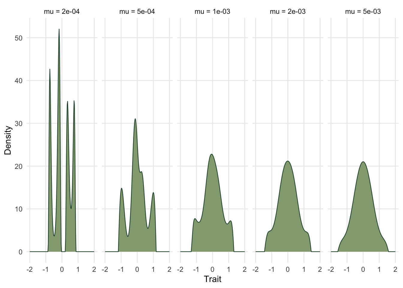
At `sigma_a = 0.8` the curvature test says branching, unambiguously. What the two counting rules see is not the same thing at all. The contiguous-block rule reports two clusters only at the lowest mutation rate and one everywhere else. The local-maximum rule reports four, four, three, one and one across the same runs.
```{r}
#| label: fig-final
#| fig-cap: "Final trait distributions at five mutation rates after 160000 steps. The same run can be read as one cluster or several depending on the rule applied."
#| fig-alt: "Five small panels of density against trait, the leftmost showing several separated peaks and the rightmost showing one broad continuous hump"
df <- do.call(rbind, lapply(seq_along(mus), function(k)
  data.frame(trait = grid, n = runs[[k]],
             mu = factor(sprintf("mu = %.0e", mus[k]),
                         levels = sprintf("mu = %.0e", mus)))))

ggplot(df, aes(trait, n)) +
  geom_area(fill = "#93a87f", colour = "#275139", linewidth = 0.4) +
  facet_wrap(~mu, nrow = 1,
             labeller = as_labeller(function(s) {
               v <- as.numeric(sub("^mu = ", "", s))
               e <- floor(log10(v) + 1e-9); m <- round(v / 10^e)
               ifelse(m == 1, paste0("mu == 10^", e), paste0("mu == ", m, " %*% 10^", e))
             }, default = label_parsed)) +
  labs(x = "Trait", y = "Density") +
  theme_minimal(base_size = 11) + te_canvas +
  theme(panel.grid.minor = element_blank())
```
The figure shows why. At low mutation the distribution is a set of narrow spikes with a genuine gap between two of them, and both rules find structure. As mutation rises the gap fills in, the distribution becomes one broad hump with internal shoulders, and the two rules diverge: the block rule sees a single connected mass while the mode rule still finds bumps in it. At the two highest rates the shoulders are still there, fainter at the highest, but they are no longer local maxima, so the mode rule too reports a single cluster.
The trait spread tells a third story. It rises steadily from `r sprintf("%.2f", res$spread[1])` to `r sprintf("%.2f", res$spread[nrow(res)])` across the mutation rates, so on that measure the population is becoming *more* diverse exactly where the block rule says branching stopped. Three defensible summaries of the same five runs point in three directions.
None of the rules is wrong. The point is that "the population branched" is not an observation, it is the output of a detection rule applied to an observation, and a paper that reports branching without stating the rule has not reported a result. The same applies to the mutation rate: it is not a nuisance parameter here, it sets whether the structure the theory predicts is resolvable at all.
## What the four checks have in common
Each failure is a mismatch between a quantity the theory is stated in and a quantity the study measures. The theory is stated in `wN` and the study reports `w`. The theory is stated for large `N` and the study runs `N = 100`. The theory predicts a curvature and the study counts peaks. The theory gives a probability of `r sprintf("%.4f", rho(1.01, 100))` and the study has 2000 replicates.
The diagnostic in every case is the same: write down the quantity the result is actually a statement about, then compute it for the specific numbers in front of you. All four checks above are a few lines of code, and all four run faster than the simulation whose interpretation they fix.
## References
Nowak, Sasaki, Taylor, Fudenberg 2004 Nature 428(6983):646-650 (10.1038/nature02414)
Geritz, Kisdi, Meszena, Metz 1998 Evolutionary Ecology 12(1):35-57 (10.1023/A:1006554906681)
Doebeli, Dieckmann 2000 The American Naturalist 156(S4):S77-S101 (10.1086/303417)
Ewens 2004 Mathematical Population Genetics 1: Theoretical Introduction, ISBN 978-0387201917
## Related tutorials
- [The Moran process and fixation probability](../the-moran-process/)
- [Evolutionary games in finite populations](../games-in-finite-populations/)
- [Adaptive dynamics and evolutionary branching](../adaptive-dynamics-and-branching/)
- [Checking a game theory model](../checking-a-game-theory-model/)