sK <- 1
K0 <- 1000
Kf <- function(x) K0 * exp(-x^2 / (2 * sK^2))
alf <- function(x, y, sa) exp(-(x - y)^2 / (2 * sa^2))

# invasion fitness of mutant y against resident x
sfit <- function(y, x, sa) 1 - alf(y, x, sa) * Kf(x) / Kf(y)Adaptive dynamics and evolutionary branching
evolutionary ecology
evolutionary game theory
population dynamics
R
ecology tutorial
Adaptive dynamics in R: invasion fitness for a Gaussian competition model, the selection gradient, pairwise invasibility plots and evolutionary branching.
Corrected 14 October 2026: the introduction said branching needs only competition that is stronger between similar phenotypes than between different ones; it now adds the condition the post derives, that competition must also be more specific than the environment is forgiving.
Corrected 1 October 2026: the equal-width case was said to make every trait combination equivalent; it now says that a resident at the singular point gives every mutant exactly zero invasion fitness, and the curvature check labels that case degenerate rather than an ESS. The link to the finite population checks said they test the branching prediction in a mutation-limited simulation; it now says what that check shows, that whether a run counts as branched depends on the mutation rate and on the counting rule.
Adaptive dynamics asks a narrow question and answers it well: given a resident population sitting at its ecological equilibrium, will a rare mutant with a slightly different trait grow? Iterating that question traces the trait through time, and the interesting part is what happens when the trajectory arrives somewhere it cannot leave.
Sometimes it stops, which is the familiar evolutionarily stable strategy. Sometimes it stops and then splits into two lineages moving apart. That second outcome, evolutionary branching, is a mechanism for the origin of diversity that needs no geographic barrier and no imposed trade-off, only competition that is stronger between similar phenotypes than between different ones and more specific than the environment is forgiving.
This post builds the standard Gaussian competition model, derives its singular point in closed form, and shows exactly which quantity decides between the two outcomes. Everything is analytic. There is no simulation and no random number in the post.
The model
Individuals carry a one-dimensional trait x, say body size or beak depth. Two things depend on it. The carrying capacity is highest at x = 0 and falls away on a Gaussian of width sigma_K, so the environment has a single best trait value. Competition between an individual of trait x and one of trait y is strongest when the traits match and decays on a Gaussian of width sigma_a.
\[ K(x) = K_0 \, e^{-x^2 / (2\sigma_K^2)}, \qquad a(x, y) = e^{-(x - y)^2 / (2\sigma_a^2)} \]
A single resident population with trait x obeys a Lotka-Volterra equation whose equilibrium density is simply K(x), because an individual competes with itself at full strength. Now introduce a mutant y at negligible density. Its per capita growth rate, the invasion fitness, is
\[ s_x(y) = 1 - \frac{a(y, x) \, K(x)}{K(y)} \]
If this is positive the mutant grows; if negative it disappears.
Note that sfit(x, x, sa) is exactly zero for any x: a mutant identical to the resident neither grows nor shrinks. That is why the sign of the invasion fitness has to be read from the first derivative, not the value.
The selection gradient
The selection gradient is the slope of invasion fitness at the resident trait. Differentiating the expression above and setting y = x, the competition term contributes nothing because the Gaussian is flat at its peak, and everything comes from the carrying capacity:
\[ D(x) = \left. \frac{\partial s_x(y)}{\partial y} \right|_{y = x} = -\frac{x}{\sigma_K^2} \]
A numerical difference confirms it.
for (x in c(-1, -0.5, 0.2, 1)) {
  num <- (sfit(x + 1e-6, x, 1.2) - sfit(x - 1e-6, x, 1.2)) / 2e-6
  cat(sprintf("x = %5.2f   numeric = %9.6f   -x/sigma_K^2 = %9.6f\n",
              x, num, -x / sK^2))
}
x = -1.00 numeric = 1.000000 -x/sigma_K^2 = 1.000000
x = -0.50 numeric = 0.500000 -x/sigma_K^2 = 0.500000
x = 0.20 numeric = -0.200000 -x/sigma_K^2 = -0.200000
x = 1.00 numeric = -1.000000 -x/sigma_K^2 = -1.000000The gradient does not depend on sigma_a at all. Whatever the shape of competition, a monomorphic population climbs the carrying-capacity curve towards x = 0 and stops there. That is the singular point, and the derivative of the gradient with respect to x is a constant negative number, so the singular point is always approached and never left. In the standard vocabulary it is convergence stable.
Convergence stability says the population gets there. It says nothing about what happens next.
Two ways to be singular
At a singular point the first derivative of invasion fitness vanishes, so the second derivative decides. Take x* = 0 and differentiate twice with respect to the mutant trait:
\[ \left. \frac{\partial^2 s_0(y)}{\partial y^2} \right|_{y = 0} = \frac{1}{\sigma_a^2} - \frac{1}{\sigma_K^2} \]
If this is negative the resident sits at a fitness maximum and no nearby mutant can invade: an evolutionarily stable strategy, and since it is also convergence stable, a continuously stable strategy. If it is positive the resident sits at a fitness minimum. The population has climbed to the worst possible place, every nearby mutant on either side can invade, and the trait distribution splits. That is a branching point.
The condition is a comparison of widths. Branching happens when sigma_a < sigma_K, that is when competition is more specific than the environment is forgiving.
for (sa in c(0.6, 0.8, 1.0, 1.2, 1.5)) {
  h <- 1e-4
  d2 <- (sfit(h, 0, sa) - 2 * sfit(0, 0, sa) + sfit(-h, 0, sa)) / h^2
  cat(sprintf("sigma_a = %.1f   curvature = %+9.6f   1/sa^2 - 1/sK^2 = %+9.6f   %s\n",
              sa, d2, 1 / sa^2 - 1 / sK^2,
              if (abs(d2) < 1e-6) "degenerate" else if (d2 > 0) "branching point" else "ESS"))
}
sigma_a = 0.6 curvature = +1.777778 1/sa^2 - 1/sK^2 = +1.777778 branching point
sigma_a = 0.8 curvature = +0.562500 1/sa^2 - 1/sK^2 = +0.562500 branching point
sigma_a = 1.0 curvature = +0.000000 1/sa^2 - 1/sK^2 = +0.000000 degenerate
sigma_a = 1.2 curvature = -0.305556 1/sa^2 - 1/sK^2 = -0.305556 ESS
sigma_a = 1.5 curvature = -0.555556 1/sa^2 - 1/sK^2 = -0.555556 ESSThe numeric second difference reproduces the closed form to six decimal places, and the switch happens exactly at sigma_a = 1, where both are zero and the model is degenerate. That degenerate case is the classical neutral one: with sigma_a equal to sigma_K a resident at the singular point gives every mutant exactly zero invasion fitness, which is why this model is usually stated with an explicit inequality rather than a limit.
Pairwise invasibility
The standard diagnostic plot puts the resident trait on the horizontal axis, the mutant trait on the vertical, and shades the sign of invasion fitness. Singular points sit where the shading meets the diagonal.
suppressMessages(library(ggplot2))
te_canvas <- theme(plot.background  = element_rect(fill = "#f5f4ee", colour = NA),
                   panel.background = element_rect(fill = "#f5f4ee", colour = NA))

gx <- seq(-1.2, 1.2, length.out = 241)
pip <- do.call(rbind, lapply(c(0.8, 1.2), function(sa) {
  g <- expand.grid(resident = gx, mutant = gx)
  g$sa <- factor(sprintf("sigma_a = %.1f", sa))
  g$sign <- ifelse(sfit(g$mutant, g$resident, sa) > 0,
                   "mutant invades", "mutant fails")
  g
}))
pip$sign <- factor(pip$sign, levels = c("mutant fails", "mutant invades"))

# the non-trivial zero contour is a straight line through the origin
for (sa in c(0.8, 1.2)) {
  slope <- (sK^2 + sa^2) / (sK^2 - sa^2)
  cat(sprintf("sigma_a = %.1f   predicted slope = %+8.4f   fitness on it = %+.3e\n",
              sa, slope, sfit(0.3 * slope, 0.3, sa)))
}
sigma_a = 0.8 predicted slope = +4.5556 fitness on it = -2.220e-16
sigma_a = 1.2 predicted slope = -5.5455 fitness on it = +0.000e+00ggplot(pip, aes(resident, mutant, fill = sign)) +
geom_raster() +
facet_wrap(~sa) +
scale_fill_manual(values = c("mutant fails" = "#e6e4dc",
"mutant invades" = "#275139")) +
geom_abline(slope = 1, intercept = 0, colour = "#8d8d80", linewidth = 0.4) +
coord_equal(expand = FALSE) +
labs(x = "Resident trait", y = "Mutant trait", fill = NULL) +
theme_minimal(base_size = 12) + te_canvas +
theme(legend.position = "top", panel.grid = element_blank())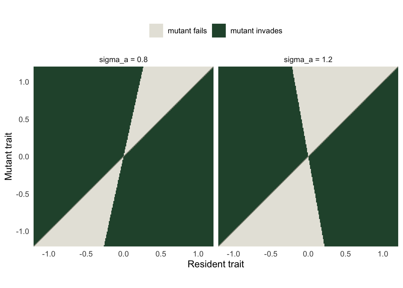
Read the plot by walking up a vertical line at a chosen resident value. Just above the diagonal, dark means an upward mutant invades and the trait moves right. Both panels show a trait converging on zero, which is the convergence stability the gradient already told us about.
The difference is at the origin, and it is a matter of which wedge pinches shut. In the left panel the pale wedges narrow to nothing as the resident approaches zero, so a resident sitting exactly at the singular point can be invaded by a mutant in either direction. In the right panel it is the dark wedges that pinch shut, and the resident at zero is safe from everything.
Setting the invasion fitness to zero gives the non-trivial boundary in closed form. It is the straight line
\[ y = x \, \frac{\sigma_K^2 + \sigma_a^2}{\sigma_K^2 - \sigma_a^2} \]
which has a steep positive slope while competition is narrower than the environment and flips to a negative slope once it is broader. The sign of that denominator is the classification, and it is the same comparison the curvature made.
A trap: mutual invasibility does not decide it
A pair of traits either side of the singular point can coexist if each can invade the other. It is tempting to use that as the branching test. In this model the test is useless, and it is worth seeing why.
for (sa in c(1.2, 0.8)) {
  for (d in c(0.05, 0.1, 0.2)) {
    cat(sprintf("sigma_a = %.1f  d = %.2f   s(-d -> +d) = %+.6f   s(+d -> -d) = %+.6f   %s\n",
                sa, d, sfit(d, -d, sa), sfit(-d, d, sa),
                if (sfit(d, -d, sa) > 0 && sfit(-d, d, sa) > 0)
                  "mutually invasible" else "not"))
  }
}
sigma_a = 1.2 d = 0.05 s(-d -> +d) = +0.003466 s(+d -> -d) = +0.003466 mutually invasible
sigma_a = 1.2 d = 0.10 s(-d -> +d) = +0.013793 s(+d -> -d) = +0.013793 mutually invasible
sigma_a = 1.2 d = 0.20 s(-d -> +d) = +0.054041 s(+d -> -d) = +0.054041 mutually invasible
sigma_a = 0.8 d = 0.05 s(-d -> +d) = +0.007782 s(+d -> -d) = +0.007782 mutually invasible
sigma_a = 0.8 d = 0.10 s(-d -> +d) = +0.030767 s(+d -> -d) = +0.030767 mutually invasible
sigma_a = 0.8 d = 0.20 s(-d -> +d) = +0.117503 s(+d -> -d) = +0.117503 mutually invasibleEvery combination is mutually invasible, including the case that the curvature calls an ESS. The reason is structural. With x = -d and y = +d the carrying capacities are equal by symmetry, so the fitness reduces to 1 - a(2d), which is positive for any nonzero separation and any width. Symmetric pairs always coexist here. The curvature is the discriminating condition; mutual invasibility of a symmetric pair is not.
After branching
Once the population is dimorphic, invasion fitness has to be computed against the joint equilibrium of both residents rather than against a single one. That equilibrium solves a small linear system.
neq <- function(x, sa) as.numeric(solve(outer(x, x, alf, sa = sa), Kf(x)))
sfit2 <- function(y, x, sa) 1 - sum(alf(y, x, sa) * neq(x, sa)) / Kf(y)

# gradient acting on the upper branch of a symmetric pair at +/- d
grad2 <- function(d, sa) {
  h <- 1e-6
  (sfit2(d + h, c(-d, d), sa) - sfit2(d - h, c(-d, d), sa)) / (2 * h)
}

for (sa in c(0.8, 0.5)) {
  r <- uniroot(grad2, c(0.05, 3), sa = sa, tol = 1e-10)$root
  n <- neq(c(-r, r), sa)
  cat(sprintf("sigma_a = %.1f   dimorphic singular pair at +/- %.6f   density %.2f each\n",
              sa, r, n[1]))
}
sigma_a = 0.8 dimorphic singular pair at +/- 0.491128 density 602.74 each
sigma_a = 0.5 dimorphic singular pair at +/- 0.493192 density 774.80 eachThe two branches separate until they reach a spacing where each stops pushing the other away, and they settle there. For sigma_a = 0.8 that spacing is 0.491128 either side of the origin, with each branch carrying 602.74 individuals. Narrowing competition to sigma_a = 0.5 moves the branches only slightly, to 0.493192, but raises the density of each to 774.80 because more distinct phenotypes compete less.
The spacing has a closed form. Setting the dimorphic gradient to zero and solving gives
\[ d^* = \sigma_a \sqrt{\tfrac{1}{2}\ln\!\left(\frac{2\sigma_K^2 - \sigma_a^2}{\sigma_a^2}\right)} \]
which exists only while sigma_a is smaller than sigma_K, the same condition as branching.
dstar <- function(sa, sK. = sK) sa * sqrt(log((2 * sK.^2 - sa^2) / sa^2) / 2)

for (sa in c(0.5, 0.8, 1.0, 1.2)) {
  ok <- 2 * sK^2 - sa^2 > sa^2
  cat(sprintf("sigma_a = %.1f   d* = %s\n", sa,
              if (ok) sprintf("%.6f", dstar(sa)) else "none"))
}
sigma_a = 0.5 d* = 0.493192
sigma_a = 0.8 d* = 0.491128
sigma_a = 1.0 d* = none
sigma_a = 1.2 d* = noneThe closed form agrees with the numerical root to six decimal places for both widths, which is the check that matters: a closed form nobody has tested against the machinery it came from is a hypothesis, not a result.
sas <- seq(0.05, 0.995, length.out = 400)
ds <- data.frame(sa = sas, d = dstar(sas))
cat("maximum spacing", round(max(ds$d), 6),
    "at sigma_a =", round(ds$sa[which.max(ds$d)], 4), "\n")
maximum spacing 0.527696 at sigma_a = 0.6611 ggplot(ds, aes(sa, d)) +
geom_line(colour = "#275139", linewidth = 1.2) +
labs(x = expression(sigma[a]), y = "Half-spacing of the two branches") +
theme_minimal(base_size = 12) + te_canvas +
theme(panel.grid.minor = element_blank())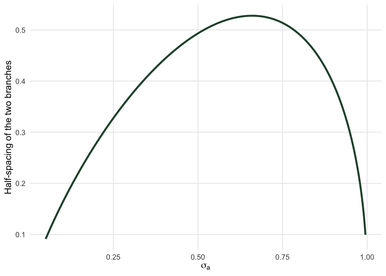
The spacing is not monotone. Very narrow competition produces branches that are close together, because a narrow kernel means the branches stop interacting after a short separation and there is nothing left to push them apart. Very broad competition produces no branching at all. The widest split comes from an intermediate width.
Branching does not stop at two
The dimorphic singular pair is itself a singular point of the dimorphic system, and the same curvature question applies to it.
for (sa in c(0.8, 0.5)) {
  r <- uniroot(grad2, c(0.05, 3), sa = sa, tol = 1e-10)$root
  h <- 1e-4
  x <- c(-r, r)
  d2 <- (sfit2(r + h, x, sa) - 2 * sfit2(r, x, sa) + sfit2(r - h, x, sa)) / h^2
  cat(sprintf("sigma_a = %.1f   curvature at the pair = %+.6f   %s\n",
              sa, d2, if (d2 > 0) "branches again" else "stable"))
}
sigma_a = 0.8 curvature at the pair = +0.049935 branches again
sigma_a = 0.5 curvature at the pair = +1.297329 branches againBoth are positive, so each branch is at a fitness minimum of its own and splits again. The curvature is much larger for the narrower kernel, 1.297329 against 0.049935, so branching cascades quickly when competition is specific and slowly when it is not. In a model with a continuous trait and no lower limit on how similar two lineages can be, the cascade never formally terminates. Real populations stop because mutation has finite step size, because population sizes become small enough for drift, and because traits run out of room.
An honest limit
The framework assumes mutations are rare and small: rare enough that the resident reaches ecological equilibrium before the next mutant appears, small enough that invasion fitness can be read off derivatives. Both assumptions fail in most real systems, and they fail in a way that matters. With larger mutations a mutant can jump past the region where the linear approximation holds and invade a resident that the gradient says is safe. With more frequent mutation the population is never monomorphic and the whole resident-mutant framing dissolves.
Invasion also guarantees nothing about replacement. Positive invasion fitness says a rare mutant grows; it does not say the resident goes extinct. Near a branching point that distinction is the entire phenomenon, because the mutant grows and the resident stays.
The model is deterministic and has no finite-population effects at all. Densities here run in the hundreds, so drift would be weak, but the branching cascade above passes through arbitrarily small differences between lineages, and at that point demographic stochasticity is doing more work than the deterministic gradient. The Moran process and fixation probability covers what finiteness does to a single locus, and Checking a finite population model shows that whether a simulated trait distribution counts as branched depends on the mutation rate and on the rule used to count clusters.
Finally, the Gaussian pair is a convenient special case, not a general result. The closed forms above depend on both kernels being Gaussian, and they should not be treated as general.
References
Geritz, Kisdi, Meszena, Metz 1998 Evolutionary Ecology 12(1):35-57 (10.1023/A:1006554906681)
Dieckmann, Doebeli 1999 Nature 400(6742):354-357 (10.1038/22521)
Metz, Nisbet, Geritz 1992 Trends in Ecology and Evolution 7(6):198-202 (10.1016/0169-5347(92)90073-K)
Doebeli, Dieckmann 2000 The American Naturalist 156(S4):S77-S101 (10.1086/303417)