Rare-species advantage and coexistence

Negative frequency dependence in R: why conspecific density dependence gives every species an edge when rare, and how the invasion criterion yields coexistence.

The previous post showed that conspecific density dependence lets two species persist, and gave the condition. This post is about why it works, in the currency that modern coexistence theory uses: negative frequency dependence. The idea is one sentence long. If every species does best when it is rare, then no species can be driven out, because falling toward extinction is exactly when it grows fastest.

Being rare is an advantage

Conspecific density dependence means a species is held back by its own abundance. Turn that around: when a species is rare, it has few conspecific neighbours, few of its specialised enemies, and so it grows faster than its competitors. Plot the difference in per-capita growth between two species against the frequency of one of them.

r0 <- 0.4; K <- 100
relgrow <- function(f1, a, Ntot = 100) {          # growth of sp1 minus sp2 at frequency f1
  N1 <- f1*Ntot; N2 <- (1 - f1)*Ntot
  r0*(1 - (N1 + a*N2)/K) - r0*(1 - (N2 + a*N1)/K)
}
c(rare_f0.1 = relgrow(0.1, 0.6), even_f0.5 = relgrow(0.5, 0.6), common_f0.9 = relgrow(0.9, 0.6))

  rare_f0.1   even_f0.5 common_f0.9 
      0.128       0.000      -0.128 

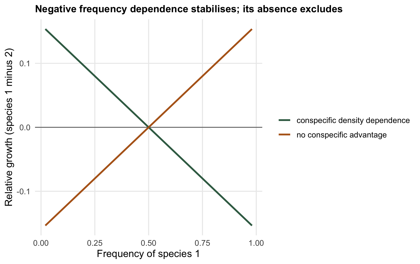
When species 1 is rare, at a frequency of 0.1, it grows faster than species 2: a positive relative growth of 0.13. When it is common, at 0.9, it grows slower, -0.13. The relative growth crosses zero at even frequencies, and it crosses with a negative slope, which is what makes the crossing stable: nudge either species away and it is pushed back. This is negative frequency dependence, and it is the formal definition of a stabilising mechanism in coexistence theory (the same family as the stabilising niche differences).

fg <- seq(0.02, 0.98, 0.02)
dn <- rbind(data.frame(f = fg, rg = sapply(fg, relgrow, a = 0.6), rule = "conspecific density dependence"),
            data.frame(f = fg, rg = sapply(fg, relgrow, a = 1.4), rule = "no conspecific advantage"))
ggplot(dn, aes(f, rg, colour = rule)) +
  geom_hline(yintercept = 0, colour = col_ref, linewidth = 0.4) +
  geom_line(linewidth = 1) +
  scale_colour_manual(values = c("conspecific density dependence" = col_cndd, "no conspecific advantage" = col_no)) +
  labs(x = "Frequency of species 1", y = "Relative growth (species 1 minus 2)", colour = NULL,
       title = "Negative frequency dependence stabilises; its absence excludes")

Figure 1: Relative growth of one species against its frequency. Under conspecific density dependence (green) it is positive when rare and negative when common, crossing zero with a negative slope, a stable coexistence point. Without it (ochre) the line slopes the wrong way and the majority always wins.

The invasion criterion

Coexistence theory turns this into a test you can run: can each species, when rare, invade a community of the other at its equilibrium? If both can, neither can be lost, and coexistence is stable; this is mutual invasibility. Compute each species’ growth rate when it is the rare invader against a resident sitting at carrying capacity.

invader_growth <- function(a) r0*(1 - a*K/K)      # growth of a rare invader vs a resident at K
c(with_cndd_a0.6 = invader_growth(0.6), no_cndd_a1.4 = invader_growth(1.4))

with_cndd_a0.6   no_cndd_a1.4 
          0.16          -0.16 

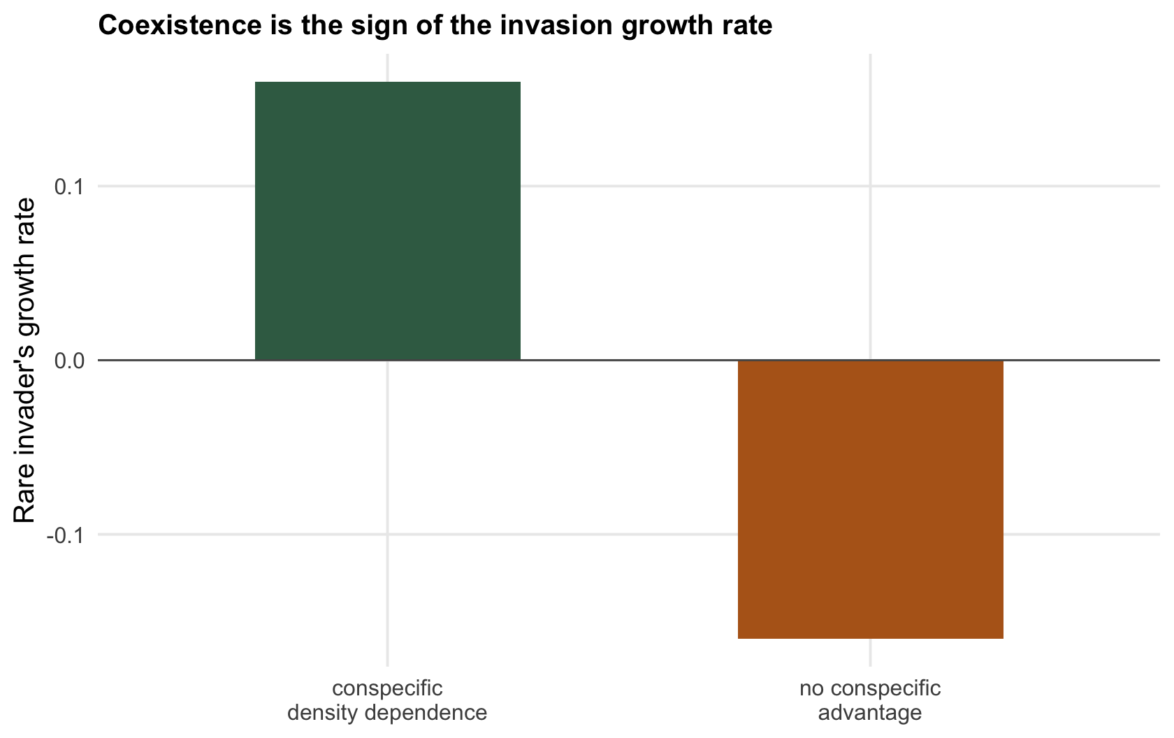
With strong conspecific density dependence the rare invader grows at +0.16: positive, so it establishes, and because the situation is symmetric both species can invade each other and coexist. Without it the invader’s growth is -0.16: negative, so the rare species cannot get a foothold and the resident holds the site alone. The whole difference between a diverse forest and a monoculture is the sign of that one number, and conspecific enemies are what flip it positive.

di <- data.frame(rule = c("conspecific\ndensity dependence", "no conspecific\nadvantage"),
                 growth = c(inv_cndd, inv_no))
ggplot(di, aes(rule, growth, fill = growth > 0)) +
  geom_col(width = 0.55) +
  geom_hline(yintercept = 0, colour = col_ref, linewidth = 0.4) +
  scale_fill_manual(values = c("TRUE" = col_cndd, "FALSE" = col_no), guide = "none") +
  labs(x = NULL, y = "Rare invader's growth rate", title = "Coexistence is the sign of the invasion growth rate")

Figure 2: Growth rate of a rare invader against a resident at carrying capacity. With conspecific density dependence (green) the invader grows, so both species invade each other and coexist; without it (ochre) the invader shrinks and is excluded.

What stabilisation still needs

Negative frequency dependence is necessary for coexistence but it is not the whole story, and it is worth being clear about the gap. Stabilisation buys a rare-species advantage, but if two species differ enough in average fitness, a large enough advantage to the stronger one, the stabilising pull may not be strong enough to overcome it, and the weaker species still loses slowly. Coexistence needs the stabilising mechanism to be large relative to the fitness difference between the species, which is the balance that modern coexistence theory makes precise. Conspecific density dependence also has to act across the whole community, not just on one convenient focal species, to explain a diverse forest. And, most practically, the frequency dependence has to be real rather than an artefact of where species happen to grow, which is exactly what the checking post is about.

Related tutorials

• Janzen-Connell and tree diversity
• Conspecific negative density dependence
• Checking a CNDD analysis
• Niche and fitness differences

References

• Comita LS et al. 2010. Science 329(5989):330-332 (10.1126/science.1190772).
• HilleRisLambers J et al. 2002. Nature 417(6890):732-735 (10.1038/nature00809).