Checking a CNDD analysis

Three checks for conspecific density dependence in R: the habitat confound that hides it, whether rarer species truly show more, and enemies versus competition.

Conspecific negative density dependence is real, important, and one of the hardest quantities in ecology to measure without fooling yourself. The pattern it predicts, worse survival among your own kind, is also produced by things that have nothing to do with density dependence, and the statistics used to estimate it carry biases that can invent it or erase it. These three checks are the ones a CNDD claim most often fails.

Check 1: is habitat confounding the density?

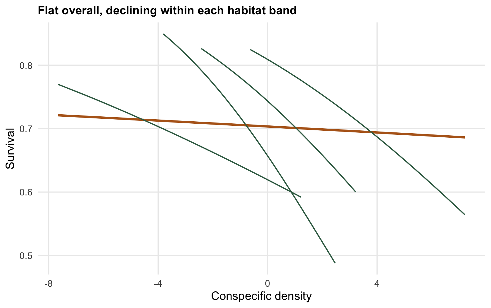
This is the big one. Species are not scattered at random; they cluster where conditions suit them. That means a seedling in a patch dense with its own kind is usually in good habitat, where survival is high, at the very moment it is surrounded by conspecifics. The habitat effect (dense conspecifics, high survival) works against the density-dependence effect (dense conspecifics, low survival), and if you ignore habitat the two can cancel.

set.seed(418); n <- 1500
habitat <- rnorm(n)
conspec <- 2*habitat + rnorm(n, 0, 1)                 # clusters in good habitat: conspec tracks habitat
surv <- rbinom(n, 1, plogis(1.0 - 0.5*conspec + 1.2*habitat))   # true CNDD is negative
c(naive = coef(glm(surv ~ conspec, family = binomial))["conspec"],
  habitat_adjusted = coef(glm(surv ~ conspec + habitat, family = binomial))["conspec"])

           naive.conspec habitat_adjusted.conspec 
             -0.01125377              -0.34806814 

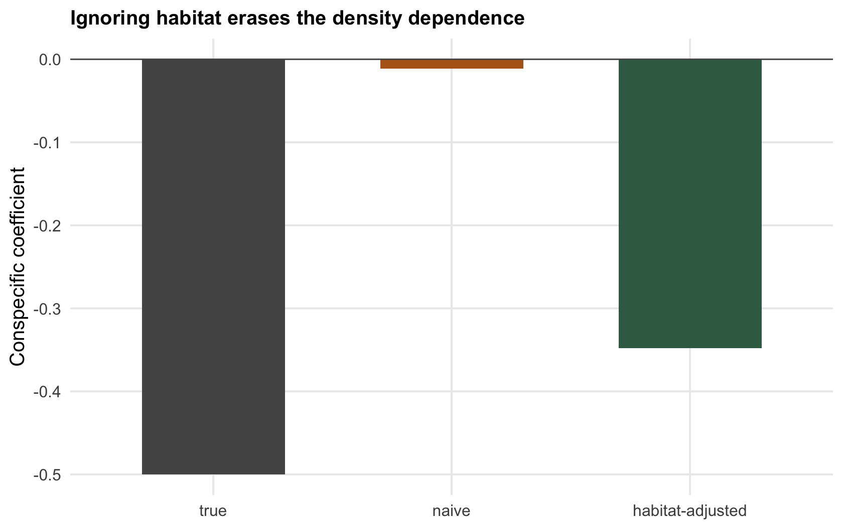
The true conspecific effect built into the data is -0.50, firmly negative. Ignore habitat and the estimated effect is -0.01, essentially zero: the density dependence has been hidden by the tendency of the species to sit in good spots. Put habitat back in and the estimate returns to -0.35, negative again. A CNDD analysis that does not control for habitat is not measuring density dependence; it is measuring where the species likes to grow, and the two are tangled by design (Detto et al. 2019 Ecology Letters 22(11):1923-1939).

dd <- data.frame(conspec = conspec, surv = surv,
                 band = cut(habitat, quantile(habitat, 0:4/4), include.lowest = TRUE, labels = paste("habitat", 1:4)))
ggplot(dd, aes(conspec, surv)) +
  geom_smooth(method = "glm", method.args = list(family = binomial), se = FALSE, colour = col_naive, linewidth = 1.1) +
  geom_smooth(aes(group = band), method = "glm", method.args = list(family = binomial), se = FALSE, colour = col_adj, linewidth = 0.6) +
  labs(x = "Conspecific density", y = "Survival",
       title = "Flat overall, declining within each habitat band")

Figure 1: Seedling survival against conspecific density. Overall (ochre) the relationship looks flat, no density dependence; split by habitat quality (green bands) it declines within every band. The confound is a Simpson’s paradox.

dc <- data.frame(est = factor(c("true","naive","habitat-adjusted"), levels = c("true","naive","habitat-adjusted")),
                 val = c(-0.5, b_naive, b_adj))
ggplot(dc, aes(est, val, fill = est)) +
  geom_col(width = 0.6) +
  geom_hline(yintercept = 0, colour = col_ref, linewidth = 0.4) +
  scale_fill_manual(values = c("true" = col_ref, "naive" = col_naive, "habitat-adjusted" = col_adj), guide = "none") +
  labs(x = NULL, y = "Conspecific coefficient", title = "Ignoring habitat erases the density dependence")

Figure 2: The estimated conspecific effect three ways. The true value is negative; the naive estimate that ignores habitat is near zero; adding habitat recovers the negative density dependence.

Check 2: do rarer species really show stronger density dependence?

A celebrated result is that rare species suffer stronger conspecific density dependence than common ones, which would explain why they stay rare (Comita et al. 2010 Science 329(5989):330-332). The pattern is probably real, but it is exactly the kind of claim the estimation can manufacture, because rare species are estimated from few individuals at low densities, where the density slope is poorly identified and its errors are large and skewed. A relationship between estimated density dependence and abundance can appear from that estimation error alone, with no difference in the underlying biology (Detto et al. 2019). The check is to confirm the pattern survives methods designed to remove the bias, and to be suspicious of any density-dependence-versus-abundance relationship that has not been tested against a null of pure estimation noise.

Check 3: is it enemies, or just competition?

Even a clean, habitat-controlled, bias-corrected conspecific effect does not prove the Janzen-Connell mechanism. Specialised enemies are one way a seedling does worse among its own kind; competition for light, water and nutrients with close relatives that need exactly the same resources is another, and both produce the same survival-against-density curve. The pattern is silent on the cause. Separating them needs manipulation, not more regression: exclude or kill the enemies with fungicide, insecticide or cages and see whether the density dependence weakens. If survival among conspecifics recovers when the pathogens are removed, enemies were the cause; if it does not, competition was. The distinction matters, because only the enemy mechanism carries the specificity that Janzen and Connell proposed.

The weight of the caveats

Three checks, and all three make the same point: a conspecific density coefficient is easy to compute and hard to earn. Habitat confounds it, estimation biases it, and its mechanism is ambiguous even when it is real. None of this means CNDD is unimportant, the diversity it can sustain is genuine, but it does mean that the strong versions of the story, that it sets abundances, that it drives the latitudinal diversity gradient, rest on measurements that need habitat controls, bias-aware methods, and ideally experiments before they carry that weight. The mechanism is one of the best ideas in community ecology and one of the easiest to measure badly.

Related tutorials

• Janzen-Connell and tree diversity
• Conspecific negative density dependence
• Rare-species advantage and coexistence
• Confounding and backdoor adjustment

References

• Comita LS et al. 2010. Science 329(5989):330-332 (10.1126/science.1190772).
• Detto M et al. 2019. Ecology Letters 22(11):1923-1939 (10.1111/ele.13372).