Conspecific negative density dependence

Conspecific negative density dependence in R: measuring how a species survives worse among its own kind, and why it stabilises coexistence.

The Janzen-Connell hypothesis makes a measurable prediction at the scale of a single seedling: it should survive worse when surrounded by its own species than by others, because its own species carries its enemies. That pattern, doing badly among your own kind, is conspecific negative density dependence, and it is the engine of the diversity result. This post measures it and shows the exact condition it has to meet to hold a community together.

Measuring it: conspecific versus heterospecific neighbours

The data are survival records for seedlings, each with a count of how many neighbours are the same species (conspecific) and how many are other species (heterospecific). Fit survival against both with a logistic regression and compare the two slopes.

set.seed(416); n <- 2000
con <- rpois(n, 4); het <- rpois(n, 8)                       # conspecific and heterospecific neighbours
surv <- rbinom(n, 1, plogis(1.2 - 0.45*con - 0.08*het))      # survival: hurt more by own kind
fit <- glm(surv ~ con + het, family = binomial)
round(coef(fit), 3)

(Intercept)         con         het 
      1.287      -0.483      -0.073 

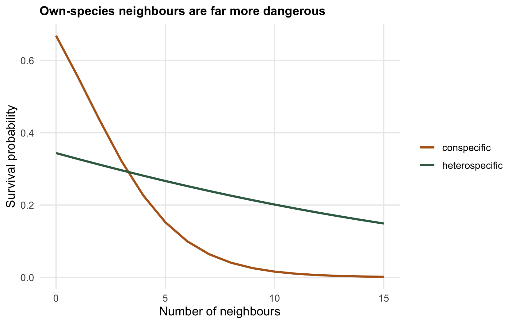
Both slopes are negative, crowding of any kind is bad, but the conspecific slope, -0.48, is several times steeper than the heterospecific one, -0.07. A seedling is punished far harder by neighbours of its own species than by an equal number of neighbours of other species. That asymmetry, not density dependence in general, is the Janzen-Connell signature, and it is what most field studies set out to estimate (Comita et al. 2010 Science 329(5989):330-332).

grid <- data.frame(d = 0:15)
pc <- rbind(data.frame(d = grid$d, p = plogis(cf[1] + cf["con"]*grid$d + cf["het"]*8), nb = "conspecific"),
            data.frame(d = grid$d, p = plogis(cf[1] + cf["con"]*4 + cf["het"]*grid$d), nb = "heterospecific"))
ggplot(pc, aes(d, p, colour = nb)) +
  geom_line(linewidth = 1) +
  scale_colour_manual(values = c("conspecific" = col_con, "heterospecific" = col_het)) +
  labs(x = "Number of neighbours", y = "Survival probability", colour = NULL,
       title = "Own-species neighbours are far more dangerous")

Figure 1: Seedling survival against neighbour density, holding the other neighbour type fixed. Survival falls steeply with conspecific neighbours (ochre) and only gently with heterospecific ones (green).

The condition for coexistence

Measuring the asymmetry is not enough; it has to be strong enough to matter. Translate it into competition between two species, where each has an effect on itself and on the other. Coexistence requires that each species limits itself more than it limits its competitor, so that whichever gets ahead is checked first. In a simple competition model that condition is the interspecific effect being weaker than the intraspecific one.

r0 <- 0.4; K <- 100
sim2 <- function(a, N0 = c(90, 10), T = 200) {
  N <- N0; for (t in 1:T) { r <- r0*(1 - (N + a*rev(N))/K); N <- pmax(N + N*r, 0) }; round(N)
}
rbind(strong_cndd_a0.6 = sim2(0.6), weak_a1.4 = sim2(1.4))

                 [,1] [,2]
strong_cndd_a0.6   63   62
weak_a1.4         100    0

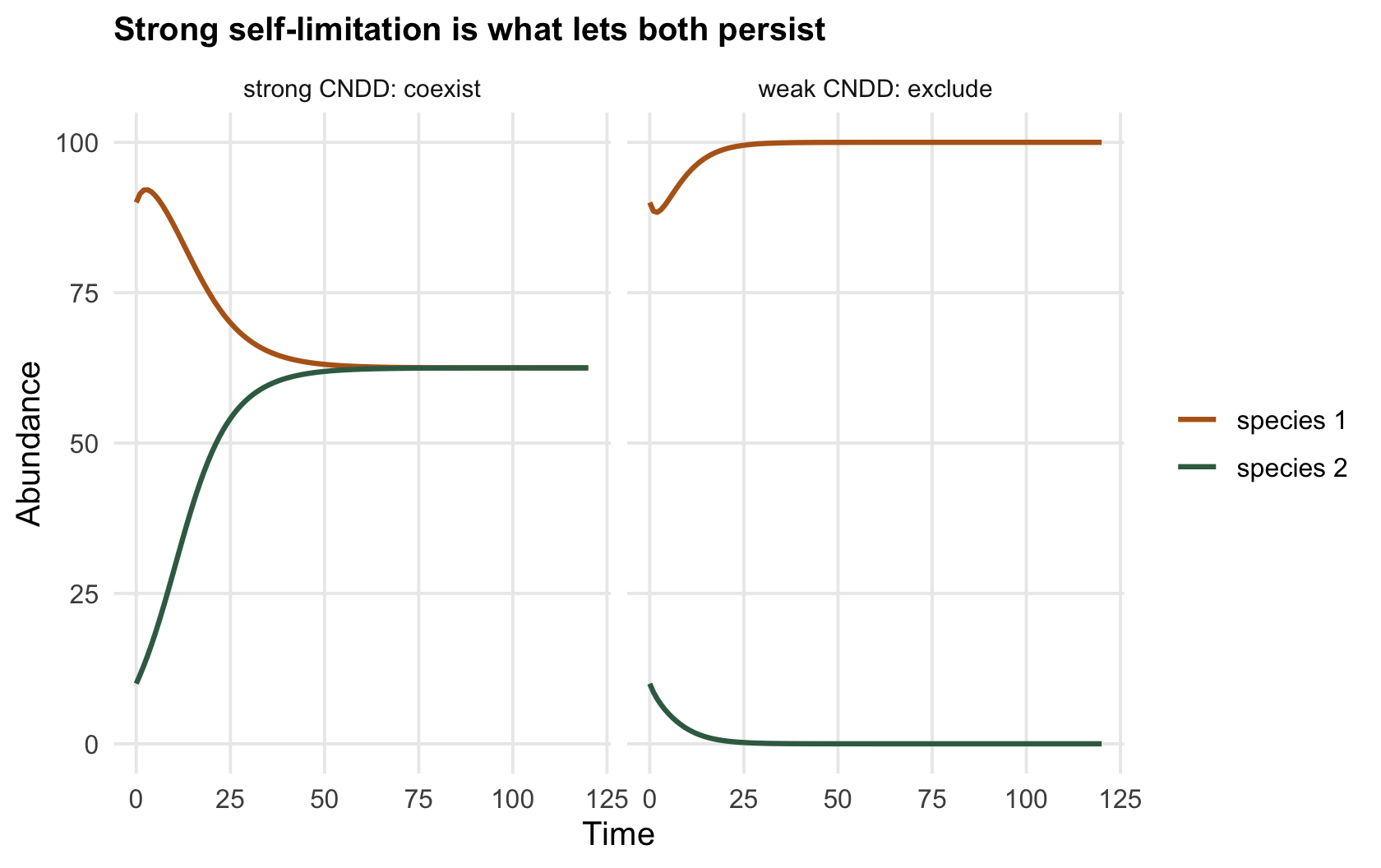
Here a is the strength of between-species competition relative to within-species. When conspecific density dependence dominates, an interspecific effect of 0.6, below one, the two species settle at 63 and 62: coexistence. When between-species competition is the stronger, 1.4, the starting majority drives the other to 0: exclusion. The Janzen-Connell mechanism matters precisely because specialised enemies push the balance toward strong self-limitation, into the coexistence side of that line.

traj <- function(a) { N <- c(90, 10); out <- data.frame(t = 0, sp1 = 90, sp2 = 10)
  for (t in 1:120) { r <- r0*(1 - (N + a*rev(N))/K); N <- pmax(N + N*r, 0); out <- rbind(out, data.frame(t = t, sp1 = N[1], sp2 = N[2])) }; out }
dd <- rbind(cbind(traj(0.6), case = "strong CNDD: coexist"), cbind(traj(1.4), case = "weak CNDD: exclude"))
dl <- reshape(dd, varying = c("sp1", "sp2"), v.names = "N", timevar = "species", direction = "long")
ggplot(dl, aes(t, N, colour = factor(species))) +
  geom_line(linewidth = 0.9) + facet_wrap(~case) +
  scale_colour_manual(values = c("1" = col_con, "2" = col_het), labels = c("species 1", "species 2")) +
  labs(x = "Time", y = "Abundance", colour = NULL, title = "Strong self-limitation is what lets both persist") +
  theme(strip.text = element_text(size = 9))

Figure 2: Two competing species over time. With strong conspecific density dependence (left) both persist; with weak conspecific relative to heterospecific competition (right) one excludes the other.

What it is and is not

Conspecific negative density dependence is the local, measurable mechanism; coexistence is the community-level consequence, and the two are not the same. A steep conspecific slope is necessary but not sufficient: it has to outweigh the between-species effect, and it has to apply across the community rather than to a single focal species. It also does not, on its own, prove that enemies are the cause; competition for a shared resource among close kin can dent survival too, and telling the mechanisms apart takes more than the slope. The coexistence logic underneath, that being rare is an advantage, is the next post, and the reasons this slope is so treacherous to estimate are the checking post.

Related tutorials

• Janzen-Connell and tree diversity
• Rare-species advantage and coexistence
• Checking a CNDD analysis
• Detecting density dependence

References

• Comita LS et al. 2010. Science 329(5989):330-332 (10.1126/science.1190772).
• Janzen DH 1970. The American Naturalist 104(940):501-528 (10.1086/282687).