---
title: "Janzen-Connell and tree diversity"
description: "The Janzen-Connell hypothesis in R: how specialised natural enemies near parent trees give rare species an edge and turn competitive exclusion into coexistence."
date: "2026-07-03 12:00"
date-modified: "2026-10-14"
categories: [ecology tutorial, R, community ecology, biodiversity, coexistence]
image: thumbnail.png
image-alt: "Species abundances under two rules: without density dependence one species dominates, with it all species coexist evenly."
---
*Corrected 14 October 2026: the post said that someone who has measured the two decay rates can tell whether escape is possible; it now adds that the mortality under the parent is needed as well.*
```{r setup}
#| code-fold: true
#| code-summary: "Setup: packages, colours and plot theme"
#| results: hide
#| message: false
#| warning: false
knitr::opts_chunk$set(echo = TRUE, message = FALSE, warning = FALSE,
                      dev = "png", dpi = 120, fig.path = "figures/",
                      fig.width = 7, fig.height = 4.4)
library(ggplot2)
theme_te <- theme_minimal(base_size = 12) +
  theme(panel.background = element_rect(fill = "#f5f4ee", colour = NA),
        plot.background  = element_rect(fill = "#f5f4ee", colour = NA),
        panel.grid.minor = element_blank(),
        plot.title = element_text(face = "bold", size = 12))
theme_set(theme_te)
col_no <- "#b5651d"; col_cndd <- "#3a6b52"; col_ref <- "#555555"

simcomm <- function(cndd, S = 8, T = 400, seed = 415) {
  set.seed(seed); f <- rep(1/S, S); fit <- runif(S, 0.9, 1.1)
  for (t in 1:T) { w <- fit * f * exp(-cndd * f); f <- w / sum(w) }
  f
}
shannon <- function(f) { f <- f[f > 0]; -sum(f * log(f)) }
f_no <- simcomm(0); f_cndd <- simcomm(6)
S_no <- sum(f_no > 0.005); S_cndd <- sum(f_cndd > 0.005)
H_no <- shannon(f_no); H_cndd <- shannon(f_cndd); Hmax <- log(8)
```
A hectare of tropical forest can hold several hundred tree species, and this is a genuine puzzle. Simple competition theory says the best competitor should win, and a species that is even slightly superior should, given time, take over. So why do so many species persist side by side, none of them running away with the forest? Janzen 1970 The American Naturalist 104(940):501-528 and Connell 1971 gave the same answer independently: the enemies of a tree do the work that competition cannot.
## Enemies that punish being common
The Janzen-Connell hypothesis is about specialised natural enemies, the seed predators, insect herbivores and soil pathogens that attack one tree species and not others. These enemies build up wherever their host is abundant, in the soil beneath a parent tree and in patches where the species is locally common. A seed or seedling landing among many of its own kind is landing in a reservoir of its own specialised enemies, and it dies at a higher rate. The result is that a species suffers most exactly where it is most common, which caps every species before it can dominate and leaves room for the rest (Connell JH 1971, in den Boer and Gradwell, Dynamics of Populations: 298-312).
Model a whole community this way. Give each species a per-capita recruitment that falls as its own frequency rises, the community-level footprint of its specialised enemies, and let the community iterate.
```{r community}
simcomm <- function(cndd, S = 8, T = 400, seed = 415) {
  set.seed(seed); f <- rep(1/S, S); fit <- runif(S, 0.9, 1.1)   # small fitness differences
  for (t in 1:T) {
    w <- fit * f * exp(-cndd * f)          # enemies cut recruitment where a species is common
    f <- w / sum(w)
  }
  f
}
round(rbind(no_enemies = simcomm(0), with_enemies = simcomm(6)), 3)
```
## Diversity from being punished
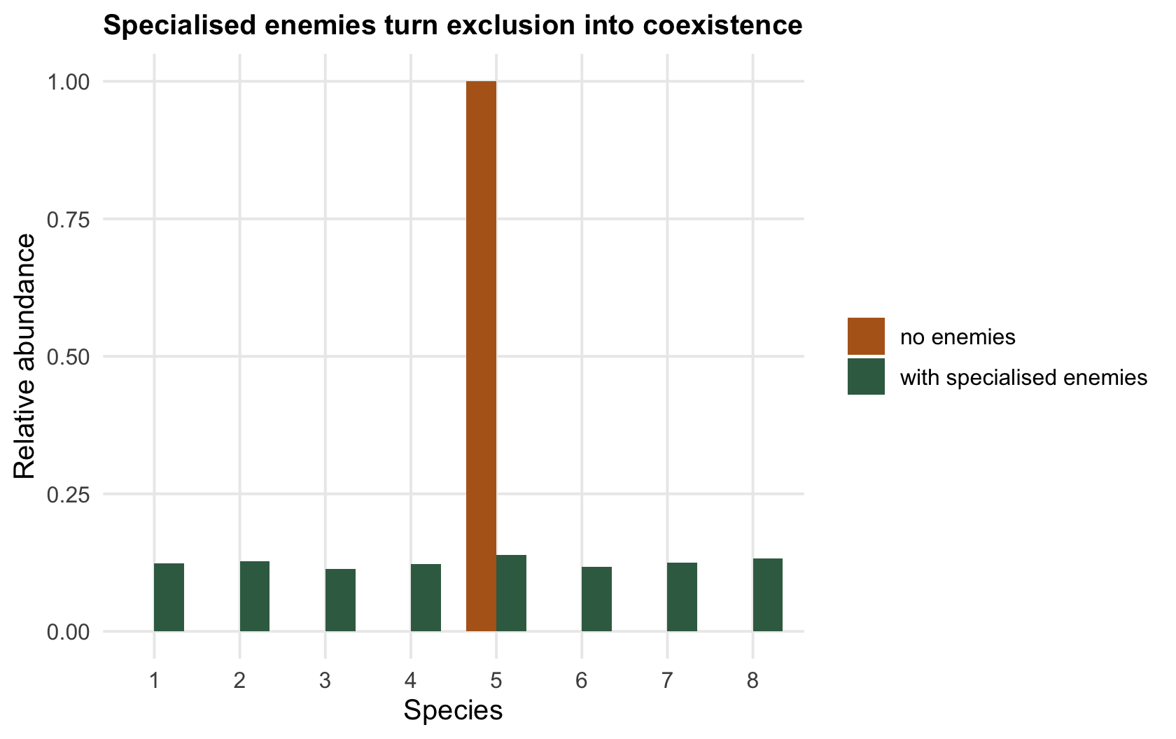
Without the density-dependent penalty, the species with the highest intrinsic fitness slowly excludes every other. Turn the enemies on and all `r sprintf("%.0f", 8)` species persist, at nearly even abundances.
```{r diversity}
shannon <- function(f) { f <- f[f > 0]; -sum(f * log(f)) }
c(species_no_enemies = sum(simcomm(0) > 0.005), shannon_no_enemies = shannon(simcomm(0)),
  species_with_enemies = sum(simcomm(6) > 0.005), shannon_with_enemies = shannon(simcomm(6)))
```
Without enemies the run above ends with `r sprintf("%.0f", S_no)` species above the threshold and a Shannon diversity of `r sprintf("%.3f", H_no)`. With them, `r sprintf("%.0f", S_cndd)` species coexist and diversity reaches `r sprintf("%.3f", H_cndd)`, which is essentially the maximum possible for this pool, `r sprintf("%.3f", Hmax)`. The same small fitness differences become harmless once every species is held back hardest when it gets ahead.
```{r fig-diversity}
#| fig-cap: "Species abundances after long competition. Without specialised enemies (ochre) one species holds almost all the abundance; with them (green) all eight coexist at even abundance."
#| fig-alt: "Two sets of bars for eight species; without enemies one bar is at one and the rest at zero, with enemies all eight bars are roughly equal."
d <- rbind(data.frame(sp = factor(1:8), f = f_no,   rule = "no enemies"),
           data.frame(sp = factor(1:8), f = f_cndd, rule = "with specialised enemies"))
ggplot(d, aes(sp, f, fill = rule)) +
  geom_col(position = "dodge", width = 0.7) +
  scale_fill_manual(values = c("no enemies" = col_no, "with specialised enemies" = col_cndd)) +
  labs(x = "Species", y = "Relative abundance", fill = NULL,
       title = "Specialised enemies turn exclusion into coexistence")
```
## From one hectare to a latitude gradient
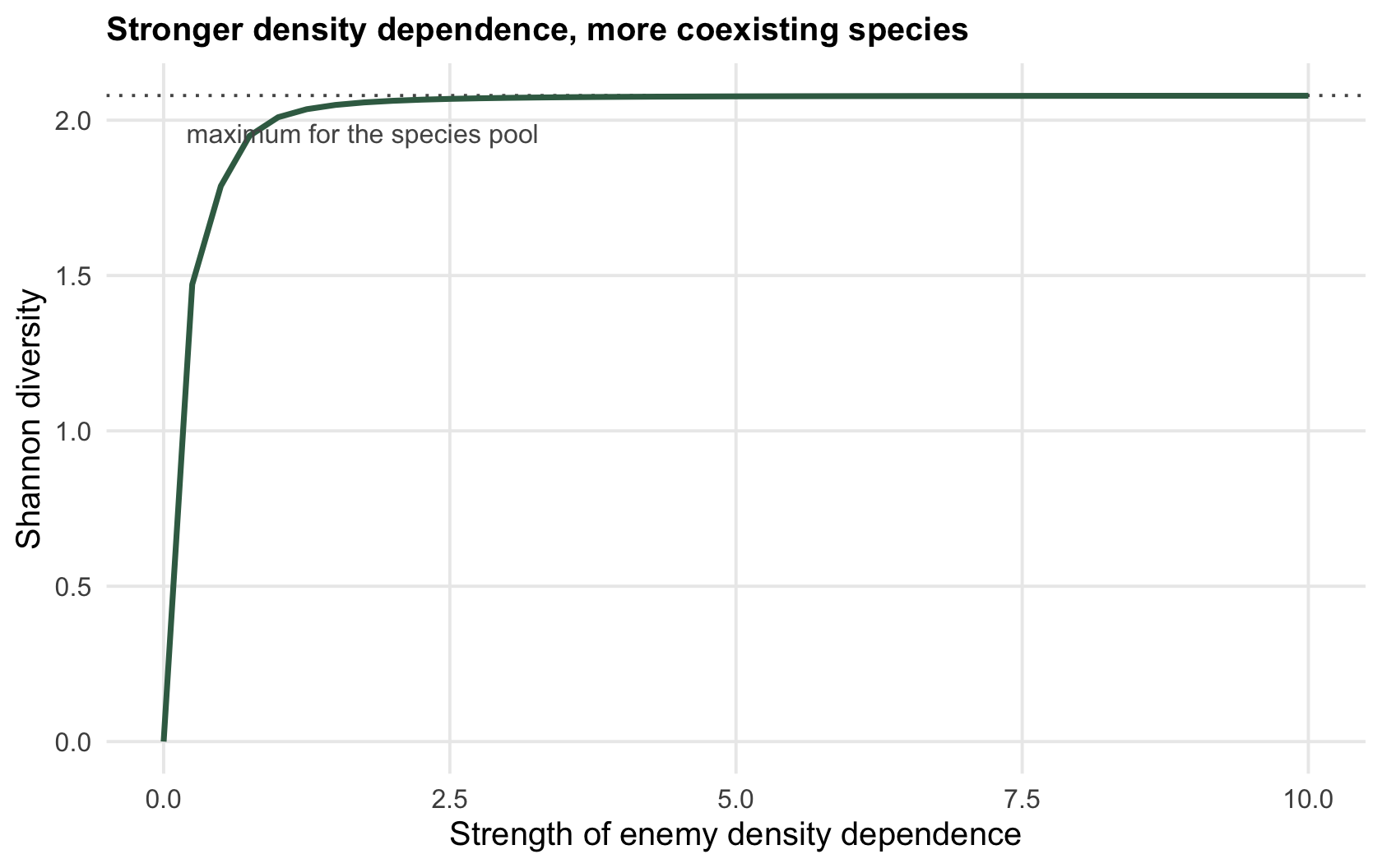
Scale the argument up and it offers an explanation for one of the oldest patterns in ecology, the increase in species richness toward the equator. If specialised enemies are more effective in warm, wet, aseasonal tropics, where pests and pathogens are never knocked back by frost or drought, then density-dependent mortality should be stronger there, and stronger density dependence supports more species. That step is the weak one. HilleRisLambers et al. 2002 Nature 417(6890):732-735 tested it in a temperate forest and found density-dependent seedling mortality just as common there as it is in tropical plots, which is not what the gradient argument predicts. Inside the model, stronger density dependence supports more diversity, up to the even community the mechanism can sustain. Whether density dependence itself strengthens toward the equator is a separate empirical claim, and it is not settled.
```{r fig-gradient}
#| fig-cap: "Community diversity against the strength of specialised-enemy density dependence. The curve starts near zero and rises as density dependence strengthens, toward the maximum for the pool."
#| fig-alt: "A rising curve of Shannon diversity against density-dependence strength, from near zero to a plateau at the maximum diversity for eight species."
cg <- data.frame(cndd = seq(0, 10, 0.25))
cg$H <- sapply(cg$cndd, function(c) shannon(simcomm(c)))
ggplot(cg, aes(cndd, H)) +
  geom_hline(yintercept = Hmax, colour = col_ref, linetype = "dotted") +
  geom_line(colour = col_cndd, linewidth = 1) +
  annotate("text", x = 3, y = Hmax - 0.12, label = "maximum for the species pool", hjust = 0, colour = col_ref, size = 3.4) +
  labs(x = "Strength of enemy density dependence", y = "Shannon diversity",
       title = "Stronger density dependence, more coexisting species")
```
## The distance a seed has to travel
Everything above runs on frequencies and has no space in it. Janzen's original argument was spatial, and it needs a second model rather than an extension of `simcomm`. Seeds fall thickest under the parent and thin out with distance. Survival does the opposite: it is worst directly under the parent, where the specialised enemies are concentrated, and it improves as a seed gets away. Recruitment is the product of the two, and the question is whether that product is largest under the parent or out at some distance from it.
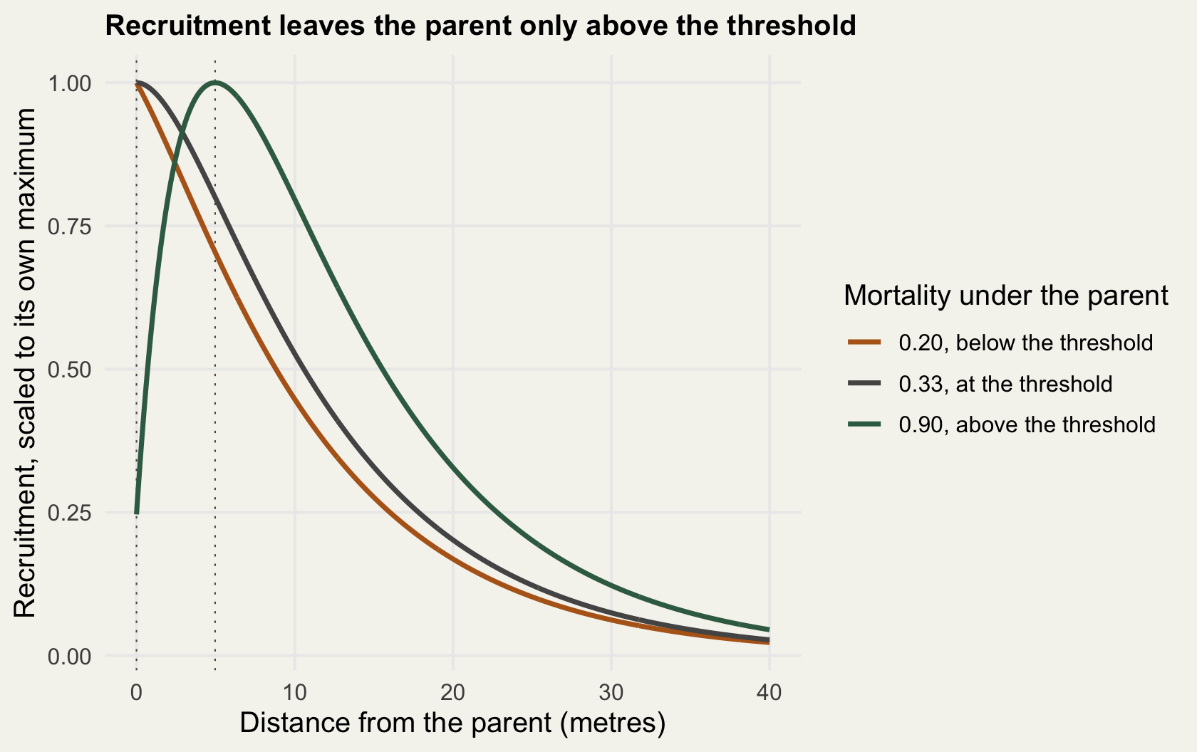
Write seed fall along a transect as `exp(-seed_decay * r)` and survival as `1 - m * exp(-enemy_decay * r)`, so `m` is the mortality directly under the parent and `enemy_decay` sets how quickly enemy pressure fades. Differentiate the product and set the distance to zero: the recruitment curve turns upward at the parent when `m * (seed_decay + enemy_decay)` is greater than `seed_decay`, so escape is possible when `m` is above `seed_decay / (seed_decay + enemy_decay)`.
What matters most about that expression is what is absent from it. No seed-shadow amplitude appears, so how many seeds the tree drops makes no difference to whether escape is possible at all. Multiply both decay rates by the same constant and the threshold does not move, so it makes no difference whether distance is counted in metres or in crown radii. Only the ratio of the two rates survives. Read the threshold the other way round and it becomes a condition on the gradient: escape needs `enemy_decay` above `seed_decay * (1 - m) / m`. What that asks of the enemy gradient depends on how deadly the ground under the parent is. The two rates have to match at a mortality of one half; below one half enemy pressure does have to fade faster than the seed shadow, and above it a gentler gradient will do, the requirement falling towards zero as mortality under the parent approaches one. A severe enough parent effect buys escape even from a survival curve that improves with distance very slowly. Someone who has measured the two decay rates, in whatever unit was convenient, and the mortality under the parent, but who knows nothing about absolute seed numbers, can still say whether escape is on the table.
```{r escape}
set.seed(703)
seed_decay  <- 0.1     # seed fall decays at this rate per metre
enemy_decay <- 0.2     # enemy pressure fades at this rate per metre
seedfall <- function(r, sd_) exp(-sd_ * r)
survival <- function(r, ed_, m) 1 - m * exp(-ed_ * r)
recruits <- function(r, sd_, ed_, m) seedfall(r, sd_) * survival(r, ed_, m)

m_star <- seed_decay / (seed_decay + enemy_decay)      # the escape threshold
peak_at <- function(m, sd_ = seed_decay, ed_ = enemy_decay) {
  g <- seq(0, 300, by = 1e-4); g[which.max(recruits(g, sd_, ed_, m))]
}
m_low   <- 0.20                                        # below the threshold
m_high  <- 0.90                                        # well above it
m_grid  <- c(m_low, 0.30, m_star, 0.40, 0.60, m_high)
esc_tab <- data.frame(
  m                = m_grid,
  peak_measured    = sapply(m_grid, peak_at),
  peak_closed_form = pmax(0, log(m_grid * (seed_decay + enemy_decay) / seed_decay) / enemy_decay))
esc_tab$survival_at_peak <- survival(esc_tab$peak_measured, enemy_decay, m_grid)
esc_tab$escape <- ifelse(m_grid > m_star, "yes", "no")
mean_dist <- 1 / seed_decay
peak_090  <- peak_at(m_high)
surv_peak <- enemy_decay / (seed_decay + enemy_decay)
print(round(esc_tab[, 1:4], 4), row.names = FALSE)
```
With a seed shadow decaying at `r sprintf("%.1f", seed_decay)` per metre, which puts the mean seed at `r sprintf("%.0f", mean_dist)` metres, and enemy pressure fading at `r sprintf("%.1f", enemy_decay)` per metre, the threshold is `r sprintf("%.4f", m_star)`. Below it the best place for a seed is directly under its parent and the peak sits at zero. Above it the peak moves out, reaching `r sprintf("%.4f", peak_090)` metres when mortality under the parent is `r sprintf("%.2f", m_high)`. The last column carries a second identity worth more than the threshold value: survival at the recruitment peak is exactly `r sprintf("%.4f", surv_peak)`, the same number in every row above the threshold, whatever `m` is. Where the peak sits depends on `m`; how dangerous the seed's position is once it gets there does not.
None of that is a finding. The threshold and the peak position are a few lines of calculus, and the grid search reproduces them to within its own step size, which is what happens when an identity is evaluated on a grid. The part the algebra does not hand over as readily is how escape behaves at the two ends of the survival gradient.
```{r escape-sweep}
set.seed(704)
m_fix  <- 0.90
b_scan <- exp(seq(log(1e-3), log(100), length.out = 4000))
r_scan <- ifelse(m_fix > seed_decay / (seed_decay + b_scan),
                 log(m_fix * (seed_decay + b_scan) / seed_decay) / b_scan, 0)
b_off  <- seed_decay * (1 - m_fix) / m_fix              # below this gradient there is no escape
b_best <- b_scan[which.max(r_scan)]
r_best <- max(r_scan)

sweep <- data.frame(enemy_decay = c(0.001, 0.01, b_off, 0.02, b_best, 0.2, 1, 50))
sweep$threshold <- seed_decay / (seed_decay + sweep$enemy_decay)
sweep$escape_distance <- ifelse(
  m_fix > sweep$threshold,
  log(m_fix * (seed_decay + sweep$enemy_decay) / seed_decay) / sweep$enemy_decay, 0)
b_soft   <- sweep$enemy_decay[4]        # a gradient flatter than the seed shadow
r_soft   <- sweep$escape_distance[4]
soft_rat <- seed_decay / b_soft
off_rat  <- seed_decay / b_off
b_far <- sweep$enemy_decay[nrow(sweep)]
thr_far <- sweep$threshold[nrow(sweep)]
r_far <- sweep$escape_distance[nrow(sweep)]
print(round(sweep, 4), row.names = FALSE)
```
Flatten the gradient and the threshold climbs towards one. With the seed shadow held fixed and mortality under the parent at `r sprintf("%.2f", m_fix)`, escape shuts off completely below an enemy decay of `r sprintf("%.4f", b_off)` per metre, which is `r sprintf("%.0f", off_rat)` times gentler than the seed shadow itself. That is the algebra above turned into numbers: a parent this deadly buys escape from a gradient far flatter than its own seed rain, and the table shows the peak already `r sprintf("%.4f", r_soft)` metres out at an enemy decay of `r sprintf("%.2f", b_soft)`, a gradient `r sprintf("%.0f", soft_rat)` times gentler than the seed shadow. Below the cutoff the survival curve barely improves with distance and offers nothing to escape to. Steepen the gradient and the threshold falls towards zero, so any mortality under the parent is enough, but the peak leaves the origin by less and less. At an enemy decay of `r sprintf("%.0f", b_far)` per metre the threshold is down to `r sprintf("%.4f", thr_far)` while the escape distance is only `r sprintf("%.4f", r_far)` metres. Escape being possible and escape reaching a distance a seed can plausibly be carried to are separate questions, and the threshold answers only the first. Between the two ends the escape distance is largest at an intermediate gradient, `r sprintf("%.2f", r_best)` metres at an enemy decay of `r sprintf("%.4f", b_best)` per metre.
```{r fig-escape}
#| fig-cap: "Recruitment against distance from the parent, each curve scaled to its own maximum. Below the threshold the best position is under the parent; at the threshold the curve is flat where it starts; above it the peak sits out at a positive distance."
#| fig-alt: "Three curves of recruitment against distance from the parent, each scaled so its highest point is one. The two lower-mortality curves start at their maximum at zero distance and fall away steadily. The high-mortality curve starts at a quarter, rises to a peak about five metres out and then declines, staying above the other two. Dotted vertical lines mark zero and the five metre peak."
m_show <- c(m_low, m_star, m_high)
lab <- sprintf("%.2f, %s the threshold", m_show, c("below", "at", "above"))
rr <- seq(0, 40, 0.05)
d_esc <- do.call(rbind, lapply(seq_along(m_show), function(i) {
  y <- recruits(rr, seed_decay, enemy_decay, m_show[i])
  data.frame(r = rr, y = y / max(y), lab = factor(lab[i], levels = lab))
}))
ggplot(d_esc, aes(r, y, colour = lab)) +
  geom_vline(xintercept = sapply(m_show, peak_at), colour = col_ref,
             linetype = "dotted", linewidth = 0.3) +
  geom_line(linewidth = 1) +
  scale_colour_manual(values = setNames(c(col_no, col_ref, col_cndd), lab)) +
  labs(x = "Distance from the parent (metres)", y = "Recruitment, scaled to its own maximum",
       colour = "Mortality under the parent",
       title = "Recruitment leaves the parent only above the threshold")
```
The model is exponential twice over and neither shape is measured here, which is the same weakness the gradient argument had. It also treats mortality under the parent and the fading of enemy pressure as properties of the tree, when both belong to the enemy community and can shift from year to year. And it is a one-tree model: nothing in it says what happens once an escaped seedling lands near a different adult of its own species, which is where the frequency model at the top of this post picks the story up.
The mechanism behind all of it is a species doing worse where it is common, which the [next post](../conspecific-negative-density-dependence/) measures directly, and its coexistence logic is negative frequency dependence, the subject of the [third post](../rare-species-advantage-and-coexistence/). Detecting it in real forests is deceptively hard, which is the [checking post](../checking-a-cndd-analysis/).
## References
- Connell JH 1971. In: den Boer PJ, Gradwell GR (eds) Dynamics of Populations. PUDOC, Wageningen: 298-312.
- HilleRisLambers J et al. 2002. Nature 417(6890):732-735 (10.1038/nature00809).
- Janzen DH 1970. The American Naturalist 104(940):501-528 (10.1086/282687).
## Related tutorials
- [Conspecific negative density dependence](../conspecific-negative-density-dependence/)
- [Rare-species advantage and coexistence](../rare-species-advantage-and-coexistence/)
- [Checking a CNDD analysis](../checking-a-cndd-analysis/)
- [Alpha diversity indices in R](../diversity-indices-in-r/)