library(ggplot2)
theme_te <- theme_minimal(base_size = 12) +
  theme(panel.grid.minor = element_blank(),
        plot.background = element_rect(fill = "#f5f4ee", colour = NA),
        panel.background = element_rect(fill = "#f5f4ee", colour = NA))

lamA <- 45; lamB <- 30                 # seeds per plant without competition
aAA <- 0.10; aBB <- 0.06               # intraspecific competition
aAB <- 0.03; aBA <- 0.06               # interspecific: B on A, and A on B
gA <- 0.60; gB <- 0.70                 # germination fractions
sA <- 0.10; sB <- 0.20 # ungerminated-seed survivalNiche and fitness differences
R
coexistence
competition
population ecology
ecology tutorial
Turn fitted annual plant competition coefficients into niche and fitness differences in R, and see why the stronger competitor need not exclude its rival.
Corrected 15 October 2026: the post said that B escapes exclusion because, when rare, it competes mostly against A rather than its own kind, and that the fitted coefficients answer the persistence question only after they are split into a niche difference and a fitness difference; it now says that B’s escape route is that A limits its own kind more than it limits B, and that the split shows why dominance and persistence give different answers.
Corrected 7 October 2026: the post said the stronger competitor ends up more abundant as it should, that its faster recovery from rarity is exactly what its fitness advantage predicts, and that A wins every head-to-head comparison in a pot; it now says the fitness ratio does not fix the abundance ranking, calls the faster recovery in line with the fitness advantage, and says A makes more seeds and presses harder on its rival.
The previous post fitted competition coefficients from a response-surface experiment. On their own, those coefficients tell you how hard each species presses on each other. They do not tell you who persists: that depends on how self-limitation compares with cross-limitation, and on how far apart the two species sit in raw competitive ability. Modern coexistence theory splits those two forces into a niche difference and a fitness difference, and the split delivers a result that raw competition data hide. A species can produce more seeds and press harder on its rival, and still fail to exclude it.
The two quantities
Take a full set of fitted coefficients for two annual plants, A and B, plus the demographic rates that close their life cycle (germination fraction \(g\), and survival of ungerminated seed in the bank \(s\)).
Two features of these numbers matter. Species A makes more seeds than B (45 against 30), and A presses harder on B than B presses on A (\(\alpha_{BA}\) = 0.06 against \(\alpha_{AB}\) = 0.03). On both counts A looks like the winner. Hold that thought.
The niche difference measures how much each species limits its own kind relative to how much it limits the other. It is built from the ratio of interspecific to intraspecific competition, pooled across the pair as a geometric mean. The complement of that pooled overlap, \(\rho\), is the stabilising niche difference:
rho    <- sqrt((aAB * aBA) / (aAA * aBB))   # niche overlap
ndiff  <- 1 - rho                            # stabilising niche difference
Show the code behind this output
rho_v <- rho; nd_v <- ndiffThe overlap is \(\rho\) = 0.548, so the niche difference is 0.452. Because the product of intraspecific coefficients (\(\alpha_{AA}\alpha_{BB}\)) exceeds the product of interspecific coefficients (\(\alpha_{AB}\alpha_{BA}\)), the two species limit themselves more, on average, than they limit each other. That is the force that stabilises coexistence: rarer species escape some competition because most of the crowding they would feel comes from their own kind, which is scarce when they are rare.
The fitness difference measures how lopsided the pair is once niche differences are set aside. It has two parts: a demographic component (who converts seeds into established plants faster over the whole life cycle) and a competitive-response component (who tolerates competition better). We write the demographic ability of each species as \(\eta\), then combine:
eta <- function(lam, g, s) g * lam / (1 - (1 - g) * s) - 1
etaA <- eta(lamA, gA, sA); etaB <- eta(lamB, gB, sB)
demo_ratio <- etaA / etaB                              # demographic component
comp_ratio <- sqrt((aBB * aBA) / (aAA * aAB))          # competitive-response component
fitness_ratio <- demo_ratio * comp_ratio               # kappa_A / kappa_B
Code behind this output; later chunks use it, so run it first
fr_v <- fitness_ratio; dr_v <- demo_ratio; cr_v <- comp_ratio; upper_v <- 1 / rhoThe fitness ratio \(\kappa_A/\kappa_B\) = 1.392 is the product of a demographic advantage (1.271) and a competitive-response advantage (1.095). Both point the same way: species A is the fitter competitor, by both routes. If competition were a simple contest, A would win.
The coexistence condition
Coexistence in this framework is a single inequality. Both species persist when their niche difference is large enough to offset their fitness difference, which happens when the fitness ratio sits below the reciprocal of the niche overlap:
\[\rho < \frac{\kappa_A}{\kappa_B} < \frac{1}{\rho}\]
upper <- 1 / rho
coexist <- (fitness_ratio > rho) && (fitness_ratio < upper)
The upper boundary is \(1/\rho\) = 1.826. The fitness ratio 1.392 falls below it, so the pair coexists. The competitively superior species is superior by less than the niche difference can absorb. Put plainly, A makes more seeds and presses harder on its rival, yet cannot drive B to zero, because A limits its own kind more than it limits B (\(\alpha_{AA}\) above \(\alpha_{BA}\)): a resident stand of A settles at a density whose crowding on a rare B plant is lighter than the crowding a resident stand of B puts on its own plants, and that gap is the escape route B needs.
The niche-fitness plane makes the margin visible. The coexistence region is the wedge between the two boundary curves; it widens as the niche difference grows. Our pair sits inside it, but not by a wide margin.
nd_seq <- seq(0.001, 0.85, length.out = 200)
band <- data.frame(nd = nd_seq, lo = 1 - nd_seq, hi = 1 / (1 - nd_seq))
ggplot(band, aes(nd)) +
  geom_ribbon(aes(ymin = lo, ymax = hi), fill = "#275139", alpha = 0.12) +
  geom_line(aes(y = hi), colour = "#275139", linewidth = 0.8) +
  geom_line(aes(y = lo), colour = "#275139", linewidth = 0.8) +
  geom_hline(yintercept = 1, linetype = "dashed", colour = "grey55") +
  annotate("point", x = nd_v, y = fr_v, colour = "#b5534e", size = 3) +
  annotate("text", x = nd_v, y = fr_v, label = "  A and B", hjust = 0,
           colour = "#b5534e", size = 3.6) +
  scale_y_log10() +
  labs(x = "niche difference (1 minus overlap)",
       y = "fitness ratio (log scale)") +
  theme_te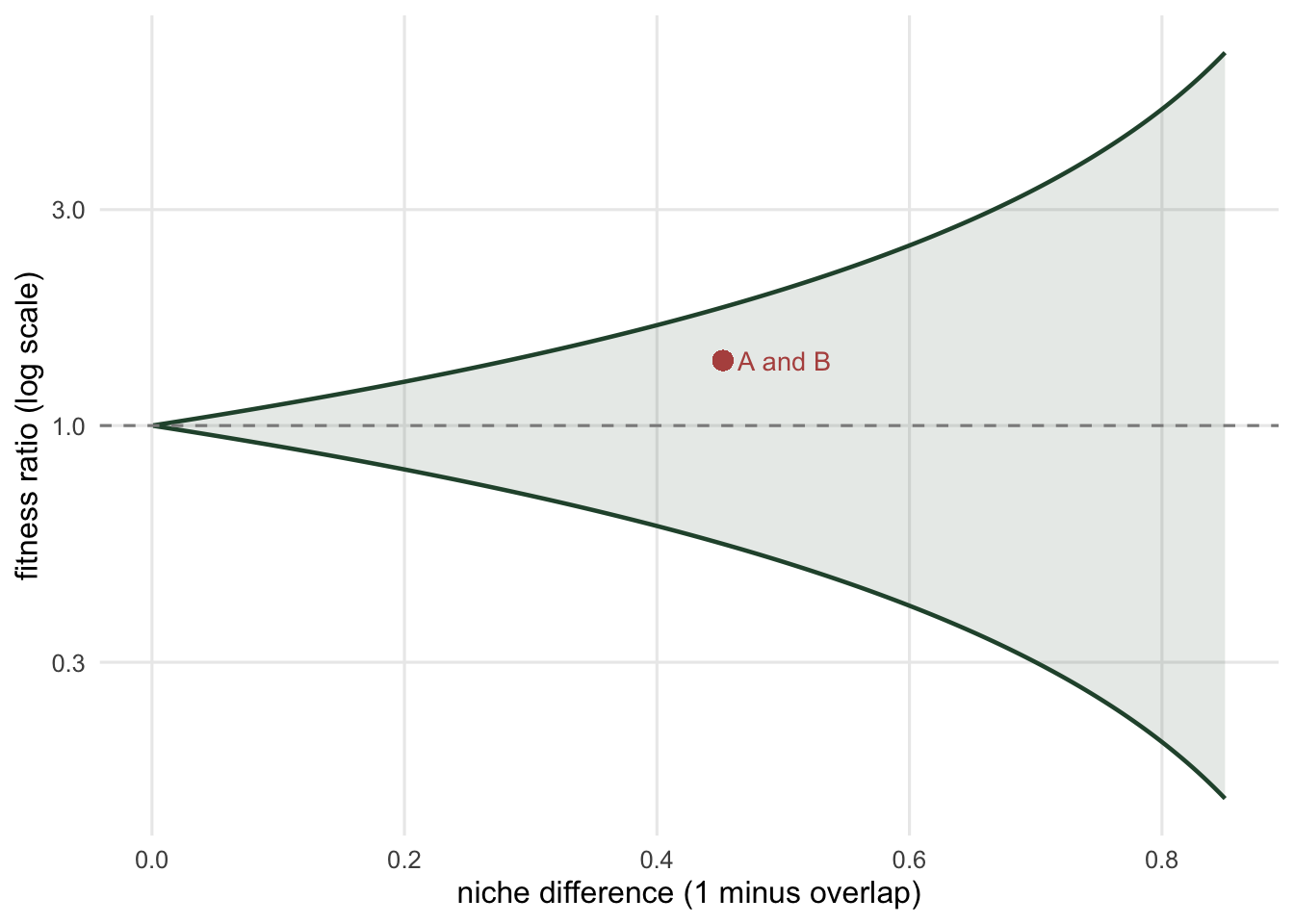
Does it actually persist? A direct check
The inequality is a shortcut for a dynamic claim: each species, introduced rare against the other at its single-species equilibrium, should grow. That is the invasion criterion, and we can test it without any of the algebra above by iterating the full two-species model.
seed_step <- function(N) {
  FA <- lamA / (1 + aAA * gA * N[1] + aAB * gB * N[2])
  FB <- lamB / (1 + aBA * gA * N[1] + aBB * gB * N[2])
  c((1 - gA) * sA * N[1] + gA * N[1] * FA,
    (1 - gB) * sB * N[2] + gB * N[2] * FB)
}
run <- function(N0, tmax = 400) {
  M <- matrix(0, tmax + 1, 2); M[1, ] <- N0
  for (t in 1:tmax) M[t + 1, ] <- seed_step(M[t, ])
  M
}
Nstar <- function(lam, g, s, a) (g * lam / (1 - (1 - g) * s) - 1) / (a * g)
NAstar <- Nstar(lamA, gA, sA, aAA); NBstar <- Nstar(lamB, gB, sB, aBB)
Introduce A rare against a resident population of B, and separately B rare against resident A. The per-capita growth rate over the first generations, on a log scale, is the invasion growth rate; positive means the invader increases.
ldgr_A <- log((1 - gA) * sA + gA * lamA / (1 + aAB * gB * NBstar))
ldgr_B <- log((1 - gB) * sB + gB * lamB / (1 + aBA * gA * NAstar))
Both invasion growth rates are positive: A into resident B gives 0.856, and B into resident A gives 0.243. Each species increases when rare, so neither can be excluded. Note that A recovers from rarity much faster than B does, in line with its fitness advantage; the point is that B still recovers at all.
Iterating from three different starting points confirms the algebra. Whether we start with A rare, B rare, or a balanced mix, the populations settle to the same interior equilibrium rather than losing a species.
tr <- rbind(
  data.frame(gen = 0:120, A = run(c(1, NBstar), 120)[, 1], B = run(c(1, NBstar), 120)[, 2], start = "A rare"),
  data.frame(gen = 0:120, A = run(c(NAstar, 1), 120)[, 1], B = run(c(NAstar, 1), 120)[, 2], start = "B rare"),
  data.frame(gen = 0:120, A = run(c(20, 20), 120)[, 1], B = run(c(20, 20), 120)[, 2], start = "balanced"))
long <- reshape(tr, varying = c("A", "B"), v.names = "N", timevar = "species",
                times = c("A", "B"), direction = "long")
ggplot(long, aes(gen, N, colour = species)) +
  geom_line(linewidth = 0.8) +
  facet_wrap(~ start) +
  scale_y_log10() +
  scale_colour_manual(values = c("A" = "#275139", "B" = "#b5534e")) +
  labs(x = "generation", y = "seed density (log scale)", colour = "species") +
  theme_te + theme(legend.position = "top")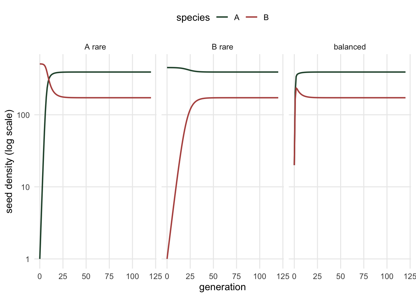
All three runs land on the same equilibrium, roughly 392 seeds of A and 172 seeds of B per plot. The stronger competitor ends up more abundant here, but the fitness ratio does not fix that: scaling up A’s per-capita effects on both species by the same factor would leave the fitness ratio and the niche overlap unchanged yet lower A’s equilibrium density, and a large enough factor would make A the rarer species. Either way, the weaker one holds a stable share. That is the substance of coexistence theory: dominance in a pot and persistence in a community are different questions, and splitting the fitted coefficients into a niche difference and a fitness difference shows why the two answers differ here.
This tidy result rests on a chain of assumptions we have not yet stressed. The invasion growth rate was evaluated at a resident density far beyond anything the fitting experiment measured, and the verdict can hinge on choices made in that extrapolation. The next post takes the analysis apart to see where the conclusion is solid and where it is fragile.
References
Chesson P 2000. Annual Review of Ecology and Systematics 31:343-366 (10.1146/annurev.ecolsys.31.1.343).
MacArthur R, Levins R 1967. American Naturalist 101(921):377-385 (10.1086/282505).
Levine JM, HilleRisLambers J 2009. Nature 461(7261):254-257 (10.1038/nature08251).
Grainger TN, Levine JM, Gilbert B 2019. Trends in Ecology and Evolution 34(10):925-935 (10.1016/j.tree.2019.05.007).