library(ggplot2)
theme_te <- theme_minimal(base_size = 12) +
  theme(panel.grid.minor = element_blank(),
        plot.background = element_rect(fill = "#f5f4ee", colour = NA),
        panel.background = element_rect(fill = "#f5f4ee", colour = NA))

lamB <- 30; aAA <- 0.10; aBB <- 0.06; aAB <- 0.03; aBA <- 0.06
gA <- 0.60; gB <- 0.70; sA <- 0.10; sB <- 0.20Checking a coexistence analysis
R
coexistence
competition
model checking
ecology tutorial
Three diagnostics for an annual plant coexistence result in R: mutual invasibility, whether your design identifies self-limitation, and stability to model form.
Corrected 14 October 2026: the post said the two competition models fit the data equally well and that the data could not separate them; it now says the Ricker fit, although Beverton-Holt generated the data, is slightly the better one, and it adds that the change of model form also turns the verdict from coexistence into the exclusion of species A.
Corrected 1 October 2026: the post said the losing species began to decline in the mixed culture only after generation ten and that a ten or fifteen generation experiment would show it thriving; it now says the decline starts right after its early peak, so such an experiment would see it declining but still present, which a presence check reads as coexistence.
The last three posts fitted competition coefficients, turned them into niche and fitness differences, and found where the coexistence verdict is fragile. This one collects the checks into a short routine you can run on your own analysis. Three questions catch most of the ways a coexistence claim goes wrong: whether a short experiment actually tested coexistence, whether your design could estimate the coefficient the verdict needs, and whether the verdict survives a reasonable change of model form.
Diagnostic 1: did a short experiment really test coexistence?
Coexistence is about the long run: each species must recover when it drifts rare. A common shortcut is to grow the two species together from an even mixture and check that both are still present after a few generations. That shortcut can pass while the pair is heading for exclusion, because a rare-when-common species is not the same as a species growing from rare. Take a pair where A clearly excludes B, and watch what a mixed culture does.
lamA <- 72                                   # A strongly superior: exclusion expected
step <- function(N) {
  FA <- lamA / (1 + aAA * gA * N[1] + aAB * gB * N[2])
  FB <- lamB / (1 + aBA * gA * N[1] + aBB * gB * N[2])
  c((1 - gA) * sA * N[1] + gA * N[1] * FA,
    (1 - gB) * sB * N[2] + gB * N[2] * FB)
}
gens <- 50
M <- matrix(0, gens + 1, 2); M[1, ] <- c(20, 20)
for (t in 1:gens) M[t + 1, ] <- step(M[t, ])
Bshare <- M[, 2] / M[1, 2]                    # B relative to its starting abundance
From an even start, B does not decline politely. It climbs to 924 per cent of its starting abundance by generation 2 and falls in every generation after that, yet is still above its starting level at generation 10 (123 per cent). Only later does it drop below where it began: 17 per cent at generation 20, and below one per cent only by generation 35. For an annual plant that is 35 years. A field experiment that ran for the ten or fifteen generations most experiments can manage would see B declining but still present, and a check that asked only whether both species persist would report coexistence.
The invasion criterion gives the right answer analytically. Introduce B rare against A at A’s single-species equilibrium and compute its growth rate:
Nstar <- function(lam, g, s, a) (g * lam / (1 - (1 - g) * s) - 1) / (a * g)
NAstar <- Nstar(lamA, gA, sA, aAA)
ldgr_B <- log((1 - gB) * sB + gB * lamB / (1 + aBA * gA * NAstar))
The invasion growth rate of B is -0.191, below zero, so B is excluded despite its early surge in the mixture. The check is not “are both species present after a while” but “does each species grow when rare”: compute the invasion growth rate directly, or run the mixture long enough to see the loser collapse, which for slow exclusion is longer than any real experiment.
df <- rbind(
  data.frame(gen = 0:gens, N = M[, 1], species = "A"),
  data.frame(gen = 0:gens, N = M[, 2], species = "B"))
ggplot(df, aes(gen, N, colour = species)) +
  annotate("rect", xmin = 0, xmax = 15, ymin = 1, ymax = Inf,
           fill = "grey85", alpha = 0.55) +
  annotate("text", x = 7.5, y = 1.4, label = "typical experiment",
           size = 3.3, colour = "grey30") +
  geom_line(linewidth = 0.9) +
  scale_y_log10(labels = scales::label_comma(drop0trailing = TRUE)) +
  scale_colour_manual(values = c("A" = "#275139", "B" = "#b5534e")) +
  labs(x = "generation", y = "seed density (log scale)", colour = "species") +
  theme_te + theme(legend.position = "top")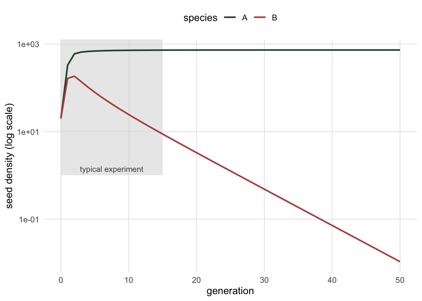
Diagnostic 2: can your design estimate self-limitation?
The verdict turns on whether intraspecific competition exceeds interspecific competition, so the intraspecific coefficient has to be estimable from your data. If conspecific density never varied, it is not, and no fitting routine will tell you the niche difference is unreliable unless you look. The test is direct: try to fit the full model on a slice of data where conspecific density is held fixed.
set.seed(207)
gp <- c(0, 2, 4, 8, 16, 32)
d <- expand.grid(Df = gp, Dh = gp); d <- d[rep(seq_len(nrow(d)), each = 6), ]
d$seeds <- rnbinom(nrow(d), mu = 45 / (1 + aAA * d$Df + aAB * d$Dh), size = 10)
additive <- d[d$Df == 0, ]                    # conspecific density fixed at zero
outcome <- tryCatch(
  nls(seeds ~ lam / (1 + aii * Df + aij * Dh), data = additive,
      start = list(lam = 40, aii = 0.05, aij = 0.05)),
  error = function(e) conditionMessage(e))
outcome
[1] "singular gradient matrix at initial parameter estimates"The singular gradient is the design telling you that self-limitation is not identified: with conspecific density fixed, the intraspecific coefficient never enters the predictions, so the data carry no information about it. A design that varied only heterospecific density gives you an interspecific coefficient and a niche difference resting on a coefficient you never estimated. If this fit fails on your data, the coexistence question is unanswerable with that data, however good the interspecific estimates look.
Diagnostic 3: does the verdict survive a change of model form?
The invasion growth rate is computed at the resident’s equilibrium, far past the fitted densities, so the competition model’s shape out there matters. Refit with a model that fits the data comparably but bends differently, and see whether the conclusions hold. Here we fit Beverton-Holt and Ricker to the same borderline pair and compare not just the verdict but the quantities the study would report.
lamA <- 52                                    # borderline pair from the previous post
simfoc <- function(seed, lam, aii, aij) {
  set.seed(seed)
  g <- expand.grid(Df = gp, Dh = gp); g <- g[rep(seq_len(nrow(g)), each = 6), ]
  g$seeds <- rnbinom(nrow(g), mu = lam / (1 + aii * g$Df + aij * g$Dh), size = 10); g
}
A <- simfoc(111, lamA, aAA, aAB)
bh <- nls(seeds ~ lam / (1 + aii * Df + aij * Dh), data = A,
          start = list(lam = 50, aii = 0.05, aij = 0.05))
rk <- nls(seeds ~ lam * exp(-aii * Df - aij * Dh), data = A,
          start = list(lam = 50, aii = 0.02, aij = 0.02))

step_A <- function(N, cf, form) {           # one year of the resident-only model
  fec <- if (form == "bh") cf["lam"] / (1 + cf["aii"] * gA * N)
       else cf["lam"] * exp(-cf["aii"] * gA * N)
  (1 - gA) * sA * N + gA * N * fec
}
fixed_pt <- function(cf, form) {            # germinated density, and its multiplier
  root <- uniroot(function(N) step_A(N, cf, form) - N, c(1, 5000))$root
  h <- 1e-4
  unname(c(gA * root,
           (step_A(root + h, cf, form) - step_A(root - h, cf, form)) / (2 * h)))
}
long_run <- function(cf, form) {            # two consecutive years after 2000 of them
  N <- 50
  for (i in 1:2000) N <- step_A(N, cf, form)
  gA * c(N, step_A(N, cf, form))
}
NBstar <- Nstar(lamB, gB, sB, aBB)          # B alone, on its own true parameters
ldgr_B <- function(NA_germ) log((1 - gB) * sB + gB * lamB / (1 + aBA * NA_germ))
ldgr_A <- function(cf, form) {
  FA <- if (form == "bh") cf["lam"] / (1 + cf["aij"] * gB * NBstar)
        else cf["lam"] * exp(-cf["aij"] * gB * NBstar)
  unname(log((1 - gA) * sA + gA * FA))
}
fp_bh <- fixed_pt(coef(bh), "bh"); fp_rk <- fixed_pt(coef(rk), "rk")
lr_bh <- long_run(coef(bh), "bh"); lr_rk <- long_run(coef(rk), "rk")
print(round(rbind(
  `Beverton-Holt` = c(fixed_point = fp_bh[1], multiplier = fp_bh[2],
                      low = min(lr_bh), high = max(lr_bh),
                      B_invades = mean(ldgr_B(lr_bh)),
                      A_invades = ldgr_A(coef(bh), "bh")),
  Ricker = c(fixed_point = fp_rk[1], multiplier = fp_rk[2],
             low = min(lr_rk), high = max(lr_rk),
             B_invades = mean(ldgr_B(lr_rk)),
             A_invades = ldgr_A(coef(rk), "rk"))), 3))
fixed_point multiplier low high B_invades A_invades
Beverton-Holt 354.683 0.071 354.683 354.683 0.003 1.065
Ricker 75.085 -2.242 9.081 170.067 1.637 -2.452The two models fit the data almost equally well (residual standard deviation 10.6 against 10.5 seeds), and the slightly better fit is the Ricker, although the data came from the Beverton-Holt model. Yet the two disagree completely on how abundant the resident is. Beverton-Holt gives species A a stable equilibrium at 355 germinated plants. The Ricker fit has no stable equilibrium at all: its fixed point sits at 75 germinated plants with a multiplier of -2.24, so the resident ends up in a two-year cycle between 9 and 170. The invasion growth rates move with the model form as well, and the verdict with them. Under Beverton-Holt they come out at 0.003 for B and 1.065 for A, so each species can invade when rare and the verdict is coexistence; under Ricker, B’s is 1.637 and A’s is -2.452, so A cannot invade and the verdict becomes the exclusion of A. The fit to these data does not pick out the model that generated them, and the choice between the two moves the reported resident abundance, the growth rates and the verdict itself.
traj <- function(cf, form, tmax = 60) {
  N <- numeric(tmax + 1); N[1] <- 50 / gA
  for (t in 1:tmax) {
    fec <- if (form == "bh") cf["lam"] / (1 + cf["aii"] * gA * N[t])
         else cf["lam"] * exp(-cf["aii"] * gA * N[t])
    N[t + 1] <- (1 - gA) * sA * N[t] + gA * N[t] * fec
  }
  gA * N
}
tf <- rbind(
  data.frame(gen = 0:60, N = traj(coef(bh), "bh"), model = "Beverton-Holt"),
  data.frame(gen = 0:60, N = traj(coef(rk), "rk"), model = "Ricker"))
ggplot(tf, aes(gen, N, colour = model)) +
  geom_line(linewidth = 1) +
  scale_y_log10() +
  scale_colour_manual(values = c("Beverton-Holt" = "#275139", "Ricker" = "#b5534e")) +
  labs(x = "generation", y = "resident A density (log scale)", colour = NULL) +
  theme_te + theme(legend.position = "top")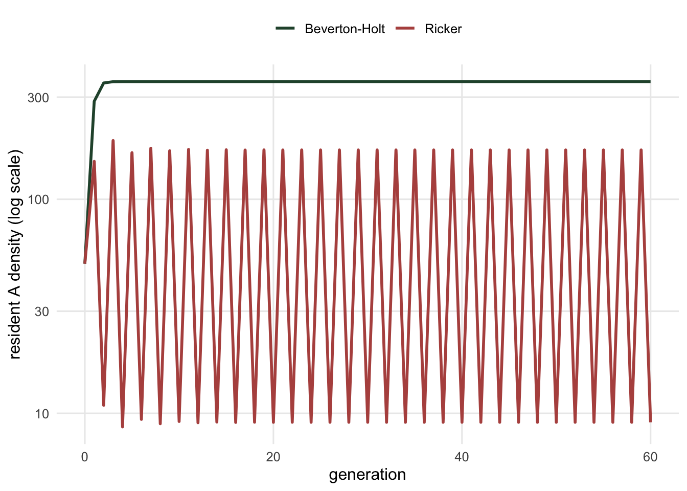
The routine
Three checks, in order. First, do not trust a short mixed culture: compute the invasion growth rate, because a pair heading for exclusion can look like coexistence for longer than an experiment runs. Second, confirm your design varied conspecific density, or the intraspecific coefficient the verdict needs is not in your data. Third, refit with a second model form and check whether the quantities you report, not just the yes-or-no verdict, hold up in the extrapolation where the invasion criterion lives. A coexistence result that clears all three is worth believing; one that clears none of them is a statement about the model, not the plants.
References
Grainger TN, Levine JM, Gilbert B 2019. Trends in Ecology and Evolution 34(10):925-935 (10.1016/j.tree.2019.05.007).
Hart SP, Freckleton RP, Levine JM 2018. Journal of Ecology 106(5):1902-1909 (10.1111/1365-2745.12954).
Levine JM, HilleRisLambers J 2009. Nature 461(7261):254-257 (10.1038/nature08251).