library(ggplot2)
theme_te <- theme_minimal(base_size = 12) +
  theme(panel.grid.minor = element_blank(),
        plot.background = element_rect(fill = "#f5f4ee", colour = NA),
        panel.background = element_rect(fill = "#f5f4ee", colour = NA))

lamA <- 52; lamB <- 30                 # A more fecund than in the previous post
aAA <- 0.10; aBB <- 0.06
aAB <- 0.03; aBA <- 0.06
gA <- 0.60; gB <- 0.70
sA <- 0.10; sB <- 0.20

rho <- sqrt((aAB * aBA) / (aAA * aBB))
eta <- function(lam, g, s) g * lam / (1 - (1 - g) * s) - 1
fitness_ratio <- (eta(lamA, gA, sA) / eta(lamB, gB, sB)) * sqrt((aBB * aBA) / (aAA * aAB))Assumptions behind coexistence
R
coexistence
competition
model checking
ecology tutorial
A coexistence verdict extrapolates far past the competition data. See in R how model form and demographic rates decide the outcome where no data constrain it.
Corrected 14 October 2026: the closing section said the fitness difference and the invasion outcome depend on a model form that the data cannot choose; it now says the data can check that form only inside the observed range, where the wrong form even fits this data set slightly better. The figure caption and alt text now say the two curves stay close inside the observed range and cross twice there, rather than being nearly indistinguishable, and the equilibrium is now compared with the largest density of either species that a focal plant experienced.
Corrected 7 October 2026: the post said the experiment measured the competition coefficients well and that the niche difference was the solid part that does not move; it now says the niche difference stays put when a demographic rate changes but rests on coefficients with sampling error, whose ratio the two fits do not agree on. It also said nothing in the observed range favoured either competition model, where the Ricker curve in fact fits slightly better although the data came from the Beverton-Holt model; the figure caption no longer says the fitted data had no heterospecific neighbours, and the largest grid density is now given per species.
The niche and fitness differences from the last post gave a clean verdict: two annual plants coexist even though one is competitively superior. That verdict came from evaluating an invasion growth rate, and an invasion growth rate is computed at the resident’s equilibrium density. Here is the uncomfortable part. That equilibrium sits far outside the range of densities the fitting experiment ever measured. The whole conclusion is an extrapolation, and two things you did not measure take over in the region where it lives: the shape of the competition model, and the demographic rates that set the equilibrium.
This post is the stress test. The niche difference depends only on the competition coefficients, so it does not move when a demographic rate changes. The fitness difference and the invasion verdict do move, and we measure by how much.
A pair near the boundary
To see fragility you need a pair near the coexistence boundary, not deep inside it. Take the same competition structure as before but raise species A’s seed output, so the pair still coexists but with little margin.
The fitness ratio is now 1.617, still below the coexistence boundary \(1/\rho\) = 1.826, but the margin is only 0.209. The pair coexists, barely. That thin margin is what the extrapolation can erase.
How far past the data does the verdict live?
The invasion growth rate of B against resident A depends on B’s fecundity when it is surrounded by A at A’s equilibrium density. So we need that equilibrium, and we need to compare it with the densities the experiment actually spanned.
Nstar <- function(lam, g, s, a) (g * lam / (1 - (1 - g) * s) - 1) / (a * g)
NAstar_seed <- Nstar(lamA, gA, sA, aAA)     # resident A, seeds per plot
NAstar_germ <- gA * NAstar_seed             # germinated A that a rare invader meets
max_data_density <- 32                       # largest neighbour count in the fitting grid
fold <- NAstar_germ / max_data_density
The fitting grid went up to 32 neighbours of each species per plot. The resident equilibrium that the invasion criterion asks about is 315 germinated plants: about 10 times beyond the largest density of either species that any focal plant in the experiment ever experienced. The verdict is not an interpolation among the data. It is a long reach past the edge of it.
The competition model is unconstrained out there
Within the observed range, the Beverton-Holt model is not the only reasonable choice. A Ricker form, where fecundity declines exponentially with density rather than hyperbolically, fits annual-plant data about as well. We simulate a response-surface experiment for focal A and fit both.
set.seed(111)
gp <- c(0, 2, 4, 8, 16, 32)
d <- expand.grid(Df = gp, Dh = gp); d <- d[rep(seq_len(nrow(d)), each = 6), ]
d$seeds <- rnbinom(nrow(d), mu = lamA / (1 + aAA * d$Df + aAB * d$Dh), size = 10)

fit_bh <- nls(seeds ~ lam / (1 + aii * Df + aij * Dh), data = d,
              start = list(lam = 50, aii = 0.05, aij = 0.05))
fit_rk <- nls(seeds ~ lam * exp(-aii * Df - aij * Dh), data = d,
              start = list(lam = 50, aii = 0.02, aij = 0.02))
sd_bh <- sd(residuals(fit_bh)); sd_rk <- sd(residuals(fit_rk))
The two models describe the observed data almost identically: the residual standard deviation is 10.60 seeds for Beverton-Holt and 10.49 for Ricker. The observed range gives no reason to prefer the Beverton-Holt model, which generated the data: if anything the Ricker curve fits slightly better. Now push both fitted curves out to the equilibrium density and watch them separate.
pred <- function(fit, model, D) {
  cf <- coef(fit)
  if (model == "bh") cf["lam"] / (1 + cf["aii"] * D) else cf["lam"] * exp(-cf["aii"] * D)
}
D_eq <- NAstar_germ
bh_eq <- pred(fit_bh, "bh", D_eq); rk_eq <- pred(fit_rk, "rk", D_eq)
gap_eq <- 100 * (rk_eq / bh_eq - 1)
At a density of 8, inside the data, the two predictions differ by 10 per cent, a gap you could not distinguish from noise. At the equilibrium density, the Beverton-Holt curve predicts 1.79 seeds per plant while the Ricker curve predicts \(3.3 \times 10^{-5}\): a ratio of about 54000 to one, which the per cent scale flattens to a meaningless 100. Note what this curve is. It is focal A’s fecundity under its own neighbours, not the invader’s fecundity, and that is the point: A’s conspecific response is what fixes where the resident settles, and the invasion criterion is then read off at whatever density that turns out to be. A gap this size does not flip the verdict by itself. It moves the density at which everything downstream is evaluated. The models agree where you have data and disagree where the verdict is computed.
xx <- exp(seq(log(1), log(D_eq * 1.2), length.out = 200))
curv <- rbind(
  data.frame(D = xx, F = pred(fit_bh, "bh", xx), model = "Beverton-Holt"),
  data.frame(D = xx, F = pred(fit_rk, "rk", xx), model = "Ricker"))
ggplot(curv, aes(D, F, colour = model)) +
  annotate("rect", xmin = 1, xmax = max_data_density, ymin = 0, ymax = Inf,
           fill = "grey85", alpha = 0.5) +
  geom_line(linewidth = 1) +
  geom_vline(xintercept = D_eq, linetype = "dashed", colour = "grey40") +
  annotate("text", x = D_eq, y = max(curv$F) * 0.9, label = "equilibrium ",
           hjust = 1, size = 3.4, colour = "grey30") +
  annotate("text", x = 6, y = max(curv$F) * 0.05, label = "observed range",
           size = 3.4, colour = "grey30") +
  scale_x_log10() +
  scale_colour_manual(values = c("Beverton-Holt" = "#275139", "Ricker" = "#b5534e")) +
  labs(x = "conspecific density (log scale)", y = "seeds per plant", colour = NULL) +
  theme_te + theme(legend.position = "top")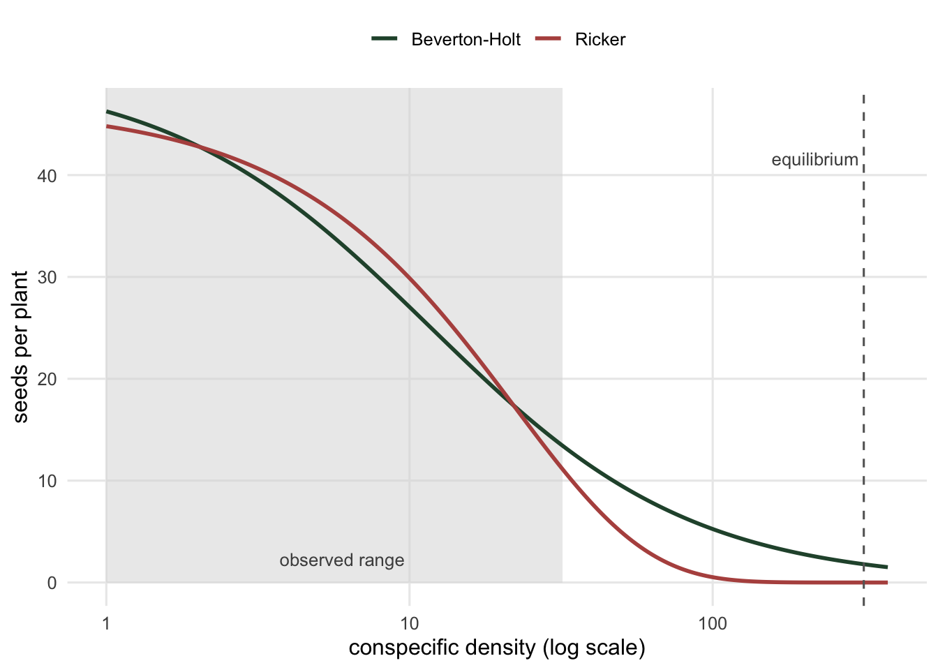
The demographic rates move it too
The niche difference depends only on the competition coefficients, which the experiment did measure, though with sampling error. The fitness difference does not: it also carries a demographic term set by germination and seed survival, and those rates are often measured separately, borrowed from another site, or assumed. Germination varies from year to year and place to place, and the verdict is sensitive to it. Sweep A’s germination fraction and track the fitness ratio against the coexistence boundary.
g_seq <- seq(0.45, 0.85, length.out = 200)
fr_g <- sapply(g_seq, function(g)
  (eta(lamA, g, sA) / eta(lamB, gB, sB)) * sqrt((aBB * aBA) / (aAA * aAB)))
g_flip <- uniroot(function(g)
  (eta(lamA, g, sA) / eta(lamB, gB, sB)) * sqrt((aBB * aBA) / (aAA * aAB)) - 1 / rho,
  c(0.45, 0.85))$root
At the baseline germination of 0.60 the pair coexists. The fitness ratio crosses the boundary at a germination of 0.681: a shift of only 0.081, well within the range germination varies across sites and years, turns the verdict from coexistence to exclusion. The competition experiment cannot protect you from this, because germination is not one of the things it measured.
gd <- data.frame(g = g_seq, fr = fr_g)
ggplot(gd, aes(g, fr)) +
  geom_hline(yintercept = 1 / rho, linetype = "dashed", colour = "#b5534e") +
  geom_line(linewidth = 1, colour = "#275139") +
  annotate("point", x = gA, y = fitness_ratio, size = 2.6, colour = "#275139") +
  annotate("text", x = 1 / rho * 0 + 0.46, y = 1 / rho + 0.03,
           label = "exclusion above this line", hjust = 0, size = 3.3, colour = "#b5534e") +
  labs(x = "germination fraction of species A", y = "fitness ratio") +
  theme_te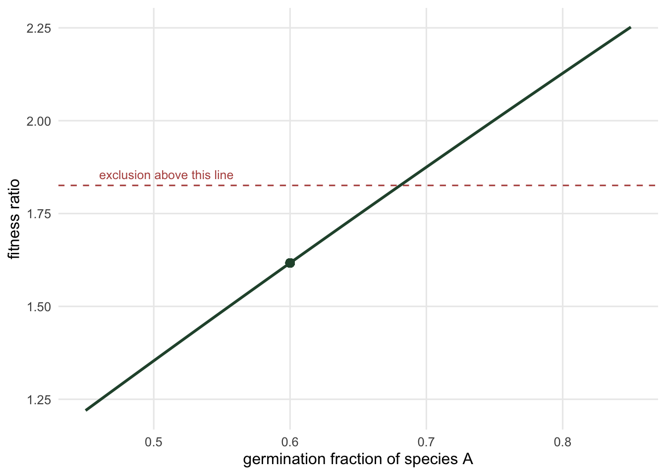
What this means for a coexistence claim
None of this says the verdict was wrong. It says the verdict rests on things the competition experiment did not constrain. The niche difference is the firmer part: it comes straight from the fitted coefficients, although those carry sampling error and the two fits above do not agree on the ratio of heterospecific to conspecific competition. The fitness difference and the invasion outcome depend on a model form that the data can check only inside the observed range, where the wrong form even fits this data set slightly better, and on demographic rates that vary. A coexistence result is only as firm as those extrapolated pieces, and near the boundary they are not firm at all. The next post turns this into a short set of checks you can run on your own analysis before you trust its verdict.
References
Hart SP, Freckleton RP, Levine JM 2018. Journal of Ecology 106(5):1902-1909 (10.1111/1365-2745.12954).
Godoy O, Kraft NJB, Levine JM 2014. Ecology Letters 17(7):836-844 (10.1111/ele.12289).
Chesson P 2000. Annual Review of Ecology and Systematics 31:343-366 (10.1146/annurev.ecolsys.31.1.343).