Spatial cross-validation for SDMs in R

Why random cross-validation overstates SDM accuracy when occurrences cluster in space, and how spatial block cross-validation gives an honest estimate, in R.

The evaluation post ended on a warning: its test sites were scattered at random across the region, so many sat right next to training points, and the reported AUC was almost certainly too high. That is spatial sorting bias, and it is the central problem this post addresses. Occurrence records cluster in space, and nearby places share environments, so a random train-test split lets a model be graded on near-copies of what it already saw. The remedy is to split the data in space rather than at random, holding out whole blocks so the test set sits some distance from the training set. This post builds spatial blocks by hand in base R and shows how much the honest estimate can differ.

library(terra)
library(mgcv)
library(dplyr)
library(tidyr)
library(ggplot2)

So far occurrence in this series depended only on temperature and precipitation, the two measured predictors, which is exactly why the model transferred well: nothing was left for space to explain. Real distributions are not so tidy. Dispersal limits, biotic interactions and unmeasured habitat all leave spatial structure that the predictors miss. To make that concrete, the simulation now adds a hidden, spatially smooth driver that the analyst never measures, and the model gains a spatial smooth term s(x, y), a common way to soak up leftover spatial pattern.

pal_paper <- "#f5f4ee"; pal_ink <- "#16241d"; pal_body <- "#2c3a31"
pal_forest <- "#275139"; pal_label <- "#46604a"; pal_line <- "#dad9ca"; pal_faint <- "#5d6b61"
pal_gold <- "#c9b458"; pal_red <- "#b5534e"
fold_cols <- c("1"="#275139","2"="#c9b458","3"="#b5534e","4"="#5d6b61","5"="#7ca2b0")
theme_te <- function(base_size = 12) {
  theme_minimal(base_size = base_size) +
    theme(text = element_text(colour = pal_body),
          plot.title = element_text(colour = pal_ink, face = "bold", size = rel(1.05)),
          plot.subtitle = element_text(colour = pal_faint),
          axis.title = element_text(colour = pal_label), axis.text = element_text(colour = pal_body),
          panel.grid.minor = element_blank(),
          panel.grid.major = element_line(colour = pal_line, linewidth = 0.3),
          strip.text = element_text(colour = pal_ink, face = "bold"),
          legend.title = element_text(colour = pal_label),
          plot.background = element_rect(fill = pal_paper, colour = NA),
          panel.background = element_rect(fill = "white", colour = NA),
          legend.key = element_rect(fill = pal_paper, colour = NA), legend.position = "top")
}
set.seed(42)
r_template <- rast(nrows = 80, ncols = 80, xmin = 0, xmax = 80, ymin = 0, ymax = 80)
xy <- xyFromCell(r_template, 1:ncell(r_template))
temp_trend <- 22 - 0.18*xy[,"y"]; tn <- rast(r_template); values(tn)<-rnorm(ncell(r_template),0,2); tn<-focal(tn,w=9,fun=mean,na.rm=TRUE)
temp <- rast(r_template); values(temp)<-temp_trend; temp<-temp+tn
prec_trend <- 500+5*xy[,"x"]; pn <- rast(r_template); values(pn)<-rnorm(ncell(r_template),0,60); pn<-focal(pn,w=9,fun=mean,na.rm=TRUE)
prec <- rast(r_template); values(prec)<-prec_trend; prec<-prec+pn
tv <- values(temp)[,1]; pv <- values(prec)[,1]
tvz <- (tv-mean(tv))/sd(tv); pvz <- (pv-mean(pv))/sd(pv)
# hidden spatially-autocorrelated driver, never measured by the analyst
set.seed(55); zr <- rast(r_template); values(zr)<-rnorm(ncell(r_template),0,1)
zr <- focal(zr, w=7, fun=mean, na.rm=TRUE); zv <- values(zr)[,1]; zv <- (zv-mean(zv,na.rm=TRUE))/sd(zv,na.rm=TRUE)
eta <- -0.5 + 0.9*(-(tvz^2)) + 0.9*(-(pvz^2)) + 4.0*zv
p_occ <- plogis(eta)
set.seed(9); site_cells <- sample(ncell(r_template), 1500)
keep <- !is.na(zv[site_cells]) & !is.na(tv[site_cells]) & !is.na(pv[site_cells]); site_cells <- site_cells[keep]
set.seed(9); y <- rbinom(length(site_cells), 1, p_occ[site_cells])
dat <- data.frame(pa = y, temp = tv[site_cells], prec = pv[site_cells], x = xy[site_cells,1], y = xy[site_cells,2])

c(sites = nrow(dat), presences = sum(dat$pa), prevalence = round(mean(dat$pa), 3))

     sites  presences prevalence 
  1500.000    485.000      0.323 

There are 1500 sites, 485 occupied, a prevalence of 0.32.

Two ways to split the same points

Random cross-validation assigns each point to one of five folds at random. Spatial block cross-validation instead overlays a grid of blocks, then assigns whole blocks to folds, so every point in a block shares its fold. Held-out points are then geographically grouped and separated from the training set, rather than interleaved with it.

k <- 5
set.seed(1); fold_rand <- sample(rep(1:k, length.out = nrow(dat)))

# spatial blocks: a grid of 20-unit cells, whole blocks assigned to folds
bs <- 20
block_id <- as.integer(factor(paste(floor(dat$x / bs), floor(dat$y / bs))))
set.seed(7); block_fold <- sample(rep(1:k, length.out = max(block_id)))
fold_sp <- block_fold[block_id]
c(blocks = max(block_id), presences_per_fold = paste(tapply(dat$pa, fold_sp, sum), collapse = ","))

            blocks presences_per_fold 
              "16" "139,112,87,76,71" 

lay <- rbind(data.frame(x=dat$x, y=dat$y, fold=factor(fold_rand), scheme="Random folds"),
             data.frame(x=dat$x, y=dat$y, fold=factor(fold_sp),   scheme="Spatial block folds"))
ggplot(lay, aes(x, y, colour = fold)) +
  geom_point(size = 0.9, alpha = 0.85) +
  facet_wrap(~scheme) +
  scale_colour_manual(values = fold_cols, name = "Fold") +
  coord_equal(expand = FALSE) +
  labs(title = "Two ways to split the same points into five folds",
       subtitle = "Random scatters folds everywhere; spatial blocking keeps each fold together",
       x = "Easting", y = "Northing") +
  theme_te(12)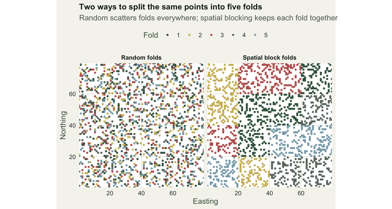

Figure 1: The same 1500 points assigned to five folds two ways.

The 20-unit grid gives 16 blocks over the region. A held-out fold under spatial blocking is a handful of whole blocks, so its points are separated from training by the block boundaries. Under random folds, every held-out point has training points as immediate neighbours.

The cost of splitting honestly

The rest is a standard k-fold loop, run once for each fold assignment. For each fold we train on the other four and predict on the held-out one, then pool all held-out predictions and compute a single AUC. Two models are compared: one with environment only, and one that adds the spatial smooth.

auc_fn <- function(sc, yy) {
  n1 <- sum(yy == 1); n0 <- sum(yy == 0)
  (sum(rank(sc)[yy == 1]) - n1 * (n1 + 1) / 2) / (n1 * n0)
}
cv_auc <- function(fold, spatial_term) {
  pr <- numeric(nrow(dat))
  form <- if (spatial_term) pa ~ s(temp) + s(prec) + s(x, y, k = 120) else pa ~ s(temp) + s(prec)
  for (f in 1:k) {
    tr <- fold != f; te <- fold == f
    m <- gam(form, data = dat[tr, ], family = binomial, method = "REML")
    pr[te] <- predict(m, dat[te, ], type = "response")
  }
  auc_fn(pr, dat$pa)
}
results <- data.frame(
  model  = rep(c("Environment only", "Environment + spatial smooth"), each = 2),
  scheme = rep(c("Random CV", "Spatial block CV"), 2),
  auc = round(c(cv_auc(fold_rand, FALSE), cv_auc(fold_sp, FALSE),
                cv_auc(fold_rand, TRUE),  cv_auc(fold_sp, TRUE)), 3))
results

                         model           scheme   auc
1             Environment only        Random CV 0.661
2             Environment only Spatial block CV 0.540
3 Environment + spatial smooth        Random CV 0.800
4 Environment + spatial smooth Spatial block CV 0.614

The pattern is the point of the post. Under random cross-validation the environment-only model scores 0.66 and the spatial-smooth model 0.80. Move to spatial blocking and both fall, to 0.54 and 0.61. The flexible model that looked clearly best under random splitting keeps only a slim edge once it is tested on genuinely new ground, because much of its apparent skill was the spatial smooth interpolating between nearby training and test points, which spatial blocking forbids.

m_full <- gam(pa ~ s(temp) + s(prec) + s(x, y, k = 120), data = dat, family = binomial, method = "REML")
round(auc_fn(predict(m_full, dat, type = "response"), dat$pa), 3)

[1] 0.852

Resubstitution, scoring the spatial-smooth model on its own training data, gives 0.85. The three numbers form a ladder of honesty: 0.85 tests on the training points, 0.80 tests on random neighbours of them, and 0.61 tests on separated blocks. Only the last estimates how the model would fare in an unsurveyed area.

results$model <- factor(results$model, levels = c("Environment only", "Environment + spatial smooth"))
ggplot(results, aes(scheme, auc, fill = scheme)) +
  geom_col(width = 0.62) +
  geom_text(aes(label = sprintf("%.3f", auc)), vjust = -0.4, colour = pal_ink, size = 3.6) +
  facet_wrap(~model) +
  scale_fill_manual(values = c("Random CV" = pal_gold, "Spatial block CV" = pal_forest), guide = "none") +
  scale_y_continuous(limits = c(0, 1), expand = expansion(mult = c(0, 0.08))) +
  labs(title = "Random cross-validation flatters both models",
       subtitle = "Spatial blocking is harder for both; the flexible spatial model falls furthest",
       x = NULL, y = "Pooled cross-validated AUC") +
  theme_te(12)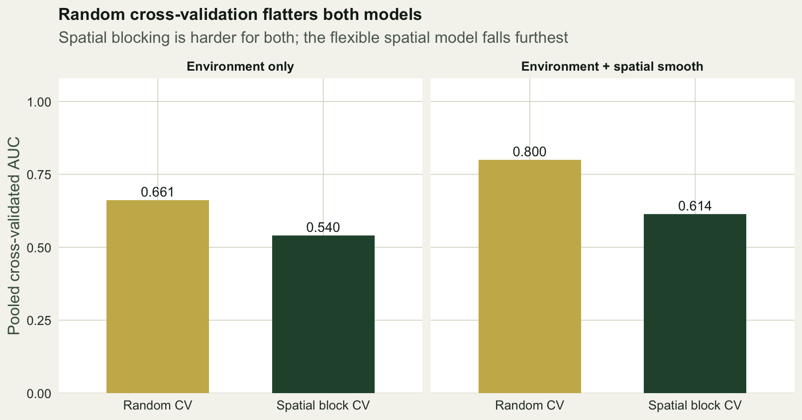

Figure 2: Pooled cross-validated AUC for both models under both splitting schemes.

Choosing block size, and when to block

Blocking works because the test blocks are larger than the range over which the data are autocorrelated, so held-out points cannot be reconstructed from their training neighbours. Blocks much smaller than that range barely separate anything; blocks so large that few remain leave too little data per fold. The practical guide is to set block size near the autocorrelation range of the predictors and residuals, which the blockCV package estimates and implements directly, along with environmental blocking and buffered leave-one-out designs (Valavi et al. 2019).

Spatial blocking is not always the right default. If the goal is to interpolate within a well-surveyed region, random cross-validation may match the intended use. But if the goal is to predict where the species occurs in unsampled areas, or under a future climate, spatial blocking is the honest test, and the recommendation is to use it whenever dependence structures exist in the data, even when the fitted model appears to account for them (Roberts et al. 2017). The same non-independence that inflates cross-validated performance here is what inflates Type-I error under pseudoreplication and drives the residual autocorrelation that Moran’s I detects: three faces of one problem. Report which scheme you used, because as the ladder above shows, the number depends on it.

References

• Guisan A, Zimmermann NE 2000. Ecological Modelling 135(2-3):147-186 (10.1016/S0304-3800(00)00354-9)
• Hijmans RJ 2012. Ecology 93(3):679-688 (10.1890/11-0826.1)
• Roberts DR et al. 2017. Ecography 40(8):913-929 (10.1111/ecog.02881)
• Valavi R, Elith J, Lahoz-Monfort JJ, Guillera-Arroita G 2019. Methods in Ecology and Evolution 10(2):225-232 (10.1111/2041-210X.13107)

Related tutorials

• Evaluating species distribution models in R
• Species distribution modelling with GLM in R
• Spatial autocorrelation and Moran’s I with spdep
• Pseudoreplication in ecology