Checking a tree ensemble

Variable importance, partial-dependence plots and the out-of-bag error all have failure modes. What they really tell you, where correlated predictors and spatial structure break them, and why prediction is not explanation.

The three previous posts built tree ensembles that predict well: bagging and the random forest by averaging, boosting by fitting residuals in sequence. This post is about the harder question of what a fitted ensemble tells you, because the standard summaries (variable importance, partial-dependence plots, and the out-of-bag error) are each easy to over-read. A forest is not a regression table. Its importance scores are not effect sizes, its partial-dependence curves are not causal, and its out-of-bag error is honest only when the data are. We show each failure on data where we know the truth, using the same hand-built forest as the earlier posts.

library(ggplot2)
te_ink<-"#16241d"; te_body<-"#2c3a31"; te_forest<-"#275139"; te_label<-"#46604a"
te_line<-"#dad9ca"; te_faint<-"#5d6b61"; te_gold<-"#cda23f"; te_red<-"#b5534e"; te_blue<-"#3f6f8f"
theme_te<-function(base_size=12){
  theme_minimal(base_size=base_size)+
  theme(text=element_text(colour=te_body),
    plot.title=element_text(colour=te_ink,size=rel(1.05)),
    plot.subtitle=element_text(colour=te_faint,size=rel(0.9)),
    axis.title=element_text(colour=te_label), axis.text=element_text(colour=te_faint),
    panel.grid.major=element_line(colour=te_line,linewidth=0.3), panel.grid.minor=element_blank(),
    plot.background=element_rect(fill="white",colour=NA), panel.background=element_rect(fill="white",colour=NA),
    legend.position="bottom", strip.text=element_text(colour=te_ink))
}
make_data <- function(n, seed){
  set.seed(seed)
  g1 <- rnorm(n); x1 <- g1+rnorm(n,0,0.6); x2 <- g1+rnorm(n,0,0.6); x3 <- g1+rnorm(n,0,0.6)
  g2 <- rnorm(n); x4 <- g2+rnorm(n,0,0.6); x5 <- g2+rnorm(n,0,0.6)
  x6 <- rnorm(n); x7 <- rnorm(n); x8 <- rnorm(n)
  f <- 2.2*(x1>0) + 0.9*x4 + 1.3*(x1>0)*(x4>0)
  data.frame(y = f + rnorm(n,0,1.1), x1,x2,x3,x4,x5,x6,x7,x8, f)
}
# hand-built random forest with impurity-gain bookkeeping (as in the bagging post, plus gain)
grow <- function(idx, dep, md, mb, mtry, gain){
  if (length(idx) < 2*mb || dep >= md) return(list(node=list(leaf=TRUE, pred=mean(yv[idx])), gain=gain))
  vars <- sample(1:ncol(X), mtry); base <- sum((yv[idx]-mean(yv[idx]))^2); best <- NULL; bg <- 1e-9
  for (v in vars){
    xs <- X[idx,v]; o <- order(xs); xo <- xs[o]; yo <- yv[idx][o]; nL <- length(idx)
    cs <- cumsum(yo); cq <- cumsum(yo^2); tot <- cs[nL]
    for (k in mb:(nL-mb)){
      if (xo[k]==xo[k+1]) next
      sL <- cs[k]; sR <- tot-sL; g <- base - (cq[k]-sL^2/k) - ((cq[nL]-cq[k])-sR^2/(nL-k))
      if (g > bg){ bg <- g; best <- list(v=v, split=(xo[k]+xo[k+1])/2, gain=g) }
    }
  }
  if (is.null(best)) return(list(node=list(leaf=TRUE, pred=mean(yv[idx])), gain=gain))
  gain[best$v] <- gain[best$v] + best$gain; go <- X[idx,best$v] <= best$split
  L <- grow(idx[go], dep+1, md, mb, mtry, gain); R <- grow(idx[!go], dep+1, md, mb, mtry, L$gain)
  list(node=list(leaf=FALSE, v=best$v, split=best$split, left=L$node, right=R$node), gain=R$gain)
}
predict1 <- function(nd, M){
  out <- numeric(nrow(M))
  for (i in seq_len(nrow(M))){ n <- nd; while (!n$leaf) n <- if (M[i,n$v] <= n$split) n$left else n$right; out[i] <- n$pred }
  out
}
predict_forest <- function(tr, M) rowMeans(sapply(tr, function(t) predict1(t, M)))
forest <- function(B, mtry, seed=21){
  set.seed(seed); n <- nrow(X); tr <- vector("list",B); oob <- vector("list",B); G <- numeric(ncol(X))
  for (b in 1:B){ ib <- sample(n,n,replace=TRUE); r <- grow(ib,0,12,5,mtry,numeric(ncol(X)))
    tr[[b]] <- r$node; G <- G + r$gain; oob[[b]] <- setdiff(1:n, ib) }
  list(trees=tr, oob=oob, imp_gain=G)
}
d <- make_data(400, 511); X <- as.matrix(d[, paste0("x",1:8)]); yv <- d$y
rf <- forest(200, mtry = 3)

Variable importance is not effect size

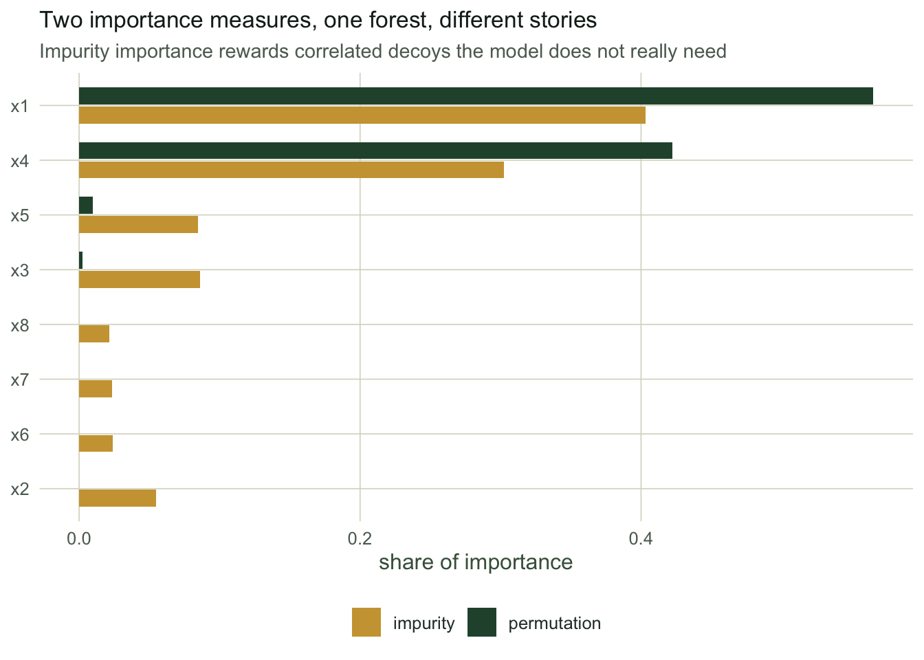
A forest offers two common importance measures and they do not agree. Impurity importance adds up how much each predictor reduced the error at the splits it was chosen for. Permutation importance shuffles a predictor in the out-of-bag data and measures how much worse the prediction gets. On our data the two real drivers are the temperature threshold (x1) and moisture (x4). The predictors x2 and x3 are correlated with x1 but have no effect of their own, and x5 is a correlated decoy for x4.

perm_imp <- function(ens){
  n <- nrow(X)
  score <- function(perm=NULL){ S <- numeric(n); C <- numeric(n)
    for (b in seq_along(ens$trees)){ ix <- ens$oob[[b]]; if (!length(ix)) next
      M <- X[ix,,drop=FALSE]; if (!is.null(perm)) M[,perm] <- X[sample(ix), perm]
      S[ix] <- S[ix] + predict1(ens$trees[[b]], M); C[ix] <- C[ix] + 1 }
    k <- C > 0; sqrt(mean((S[k]/C[k] - yv[k])^2)) }
  b0 <- score(); set.seed(3); sapply(1:8, function(j) score(j) - b0)
}
imp_gain <- rf$imp_gain / sum(rf$imp_gain)
ip <- pmax(perm_imp(rf), 0); imp_perm <- ip / sum(ip)
names(imp_gain) <- names(imp_perm) <- paste0("x",1:8)
decoy_gain <- round(100*sum(imp_gain[c("x2","x3")]), 0)
decoy_perm <- round(100*sum(imp_perm[c("x2","x3")]), 0)

Impurity importance hands the two correlated decoys x2 and x3 about 14% of the total, and it gives the pure-noise predictors a small non-zero share as well: it never quite reaches zero, and it inflates predictors that are correlated with a real driver, because in a random forest x1 is often hidden by mtry and a decoy is chosen in its place. Permutation importance leaves the same two decoys near zero and pushes the noise predictors to zero, because the forest reaches for the true driver first and shuffling a redundant decoy barely hurts. The lesson from the ecology literature is the same: prefer permutation importance to the impurity measure, and even then read it as which predictors the model leans on, not as the size or direction of an effect.

Two importance rankings of the same forest. Impurity importance credits the correlated decoys (x2, x3) and the noise predictors; permutation importance leaves them near zero. Neither is an effect size.

Partial dependence hides interactions

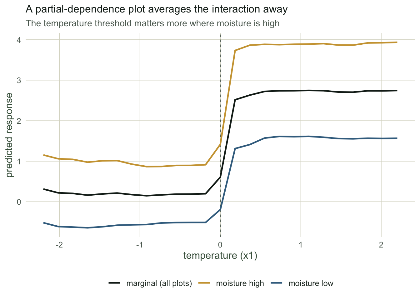
A partial-dependence plot for a predictor fixes it at a grid of values, predicts for every observation, and averages. It answers a marginal question: on average across the sample, how does the prediction move as this predictor changes. That average has two blind spots. When predictors are correlated it averages over combinations that never occur, and, more simply, it hides interactions by averaging them away. Our response has a real interaction: crossing the temperature threshold matters more where moisture is high. The marginal curve cannot show that, so we compare it with the same curve computed separately on the low-moisture and high-moisture plots.

gx <- seq(-2.2, 2.2, length.out = 25)
pdp <- function(rows, v = 1) sapply(gx, function(val){ M <- X[rows,,drop=FALSE]; M[,v] <- val; mean(predict_forest(rf$trees, M)) })
pd_marg <- pdp(seq_len(nrow(X)))
pd_lo <- pdp(which(d$x4 < 0)); pd_hi <- pdp(which(d$x4 > 0))
step_lo <- round(pd_lo[16] - pd_lo[10], 2)   # jump across the threshold, low moisture
step_hi <- round(pd_hi[16] - pd_hi[10], 2)   # jump across the threshold, high moisture

Across the threshold the prediction jumps by about 2.09 where moisture is low and by about 2.99 where moisture is high. The single marginal curve splits the difference and reports one step for everyone, which is true of no site in particular. A reader who takes the marginal partial-dependence plot as the effect of temperature would miss that the effect nearly doubles with moisture, which for a real ecological question is usually the point.

Partial dependence of the prediction on temperature. The marginal curve averages over moisture; computed separately, the threshold jump is much larger where moisture is high. The average hides the interaction.

The out-of-bag error is honest only when the data are independent

The out-of-bag error was a selling point of bagging: a free estimate of test error. It rests on the left-out plots being independent of the in-bag plots. Ecological data are usually spatially autocorrelated, so a left-out plot has near neighbours still in the training sample, and the forest can all but look up the answer. The out-of-bag error then flatters the model. To see it, we build data with a smooth spatial field the forest can exploit through the coordinates, and compare the random out-of-bag error with an error from holding out whole spatial blocks.

field <- function(sx, sy, seed){ set.seed(seed); K <- 7; grid <- matrix(rnorm(K*K),K,K); gg <- seq(0,1,length.out=K)
  i <- findInterval(sx,gg,all.inside=TRUE); j <- findInterval(sy,gg,all.inside=TRUE)
  tx <- (sx-gg[i])/(gg[i+1]-gg[i]); ty <- (sy-gg[j])/(gg[j+1]-gg[j])
  (1-tx)*(1-ty)*grid[cbind(i,j)] + tx*(1-ty)*grid[cbind(i+1,j)] + (1-tx)*ty*grid[cbind(i,j+1)] + tx*ty*grid[cbind(i+1,j+1)] }
set.seed(77); n2 <- 500; sx <- runif(n2); sy <- runif(n2); xa <- rnorm(n2); xb <- rnorm(n2)
ys <- 1.5*(xa>0) + 0.8*xb + 2.4*field(sx,sy,5) + rnorm(n2,0,0.8)
X <- as.matrix(data.frame(xa, xb, sx, sy)); yv <- ys

sf <- forest(150, mtry = 2, seed = 31)                      # random bagging: out-of-bag error
S <- numeric(n2); C <- numeric(n2)
for (b in seq_along(sf$trees)){ ix <- sf$oob[[b]]; S[ix] <- S[ix] + predict1(sf$trees[[b]], X[ix,,drop=FALSE]); C[ix] <- C[ix] + 1 }
k <- C > 0; oob_err <- sqrt(mean((S[k]/C[k] - yv[k])^2))

blk <- (cut(sx,4,labels=FALSE)-1)*4 + cut(sy,4,labels=FALSE) # hold out 4x4 spatial blocks
pe <- numeric(0); ye <- numeric(0)
for (b in sort(unique(blk))){ tst <- which(blk==b); trn <- which(blk!=b); nn <- length(trn)
  set.seed(200+b); tt <- lapply(1:100, function(z) grow(sample(trn,nn,replace=TRUE),0,12,5,2,numeric(ncol(X)))$node)
  pe <- c(pe, predict_forest(tt, X[tst,,drop=FALSE])); ye <- c(ye, yv[tst]) }
cv_err <- sqrt(mean((pe - ye)^2))
oob_r <- round(oob_err,2); cv_r <- round(cv_err,2); gap <- round(100*(cv_err-oob_err)/cv_err, 0)

The out-of-bag error is 1.47, but the spatially blocked error is 1.91: the free estimate understates the error by about 23% because nearby plots leak across the split. On spatially structured data this is the rule, not a corner case, and it is the same problem the spatial cross-validation post raised for distribution models. Report a blocked error, not the out-of-bag number, whenever location carries information.

Prediction is not explanation

None of this is an argument against tree ensembles. They are among the best off-the-shelf predictors for messy ecological data, and the boosted-regression-tree guides earned their place for good reason. It is an argument about reading them. A forest fits a flexible function of its inputs, tuned by choices you made (the tree depth, mtry, the learning rate, the number of trees), and every summary you draw from it describes that fitted function, not the ecology. Variable importance ranks what the function uses and is biased by correlation; a partial-dependence plot shows a marginal slice and averages interactions away; the out-of-bag error is optimistic under the spatial structure most ecological data carry. A model built and validated to predict answers a different question from one built to explain, and the two are easy to confuse precisely because the same forest can look like it answers both. When the goal is to understand a mechanism, the honest path is a blocked-validation estimate of how well it predicts, permutation or conditional importance read as reliance rather than effect, and the causal question handled by the tools built for it.

That closes this series on trees and ensembles: a single tree, its bagged and random-forest averages, boosting, and how to check the result without fooling yourself.

References

• Strobl, Boulesteix, Zeileis, Hothorn 2007 BMC Bioinformatics 8:25 (10.1186/1471-2105-8-25).
• Strobl, Boulesteix, Kneib, Augustin, Zeileis 2008 BMC Bioinformatics 9:307 (10.1186/1471-2105-9-307).
• Shmueli 2010 Statistical Science 25(3):289-310 (10.1214/10-STS330).
• Roberts, Bahn, Ciuti, Boyce, Elith and others 2017 Ecography 40(8):913-929 (10.1111/ecog.02881).
• Molnar 2022 Interpretable Machine Learning: A Guide for Making Black Box Models Explainable (2nd ed), christophm.github.io/interpretable-ml-book.

Related tutorials

• Boosted regression trees
• Bagging and random forests
• Regression trees and CART
• Spatial cross-validation for distribution models