Bagging and random forests, by hand

Why averaging bootstrapped trees cuts variance, how the out-of-bag error gives a free honest estimate, and what the mtry trick in a random forest actually buys, built from scratch in R.

A single regression tree is unstable: the previous post showed that resampling the data changes the splits, and that the tree is a high-variance estimator. There is a general cure for variance. If you have many noisy estimates of the same thing, average them. Bagging does exactly that with trees, the random forest sharpens it, and both give a free estimate of their own error along the way. We build all of it from scratch so that nothing is hidden inside a package.

The same problem, more predictors

To make the averaging worth doing we need a problem with several predictors, some of them correlated, since correlation is where the random forest earns its keep. The response is driven by a temperature threshold and a moisture gradient, with an interaction. Two more predictors are correlated with temperature but have no direct effect, one is correlated with moisture, and three are pure noise.

library(ggplot2)
te_ink<-"#16241d"; te_body<-"#2c3a31"; te_forest<-"#275139"; te_label<-"#46604a"
te_paper<-"#f5f4ee"; te_line<-"#dad9ca"; te_faint<-"#5d6b61"
te_gold<-"#cda23f"; te_green<-"#2f8f63"; te_red<-"#b5534e"; te_lowc<-"#c9b458"; te_highc<-"#1d5b4e"
theme_te<-function(base_size=12){
  theme_minimal(base_size=base_size)+
  theme(text=element_text(colour=te_body),
    plot.title=element_text(colour=te_ink,size=rel(1.05)),
    plot.subtitle=element_text(colour=te_faint,size=rel(0.9)),
    axis.title=element_text(colour=te_label), axis.text=element_text(colour=te_faint),
    panel.grid.major=element_line(colour=te_line,linewidth=0.3), panel.grid.minor=element_blank(),
    plot.background=element_rect(fill="white",colour=NA), panel.background=element_rect(fill="white",colour=NA),
    legend.position="bottom", strip.text=element_text(colour=te_ink))
}

make_data <- function(n, seed){
  set.seed(seed)
  g1 <- rnorm(n); x1 <- g1 + rnorm(n,0,0.6); x2 <- g1 + rnorm(n,0,0.6); x3 <- g1 + rnorm(n,0,0.6)
  g2 <- rnorm(n); x4 <- g2 + rnorm(n,0,0.6); x5 <- g2 + rnorm(n,0,0.6)
  x6 <- rnorm(n); x7 <- rnorm(n); x8 <- rnorm(n)
  f <- 2.2*(x1 > 0) + 0.9*x4 + 1.3*(x1 > 0)*(x4 > 0)
  y <- f + rnorm(n, 0, 1.1)
  data.frame(y, x1, x2, x3, x4, x5, x6, x7, x8, f)
}
d  <- make_data(400, 511)
te <- make_data(4000, 999)   # large independent test set
X <- as.matrix(d[, paste0("x",1:8)]); Xte <- as.matrix(te[, paste0("x",1:8)]); yv <- d$y
rmse <- function(a,b) sqrt(mean((a-b)^2))
noise_floor <- rmse(te$f, te$y)

One tree builder, two ensembles

A random forest is bagging plus one extra idea. In bagging, every tree sees a bootstrap resample of the plots and is grown deep. In a random forest, each tree does the same but at every split it may only choose among a random subset of mtry predictors, not all of them. That single restriction is the whole difference, so we write one tree function that takes mtry and use it for both: mtry equal to all eight predictors is bagging, mtry equal to three is a random forest.

grow1 <- function(idx, depth, maxdepth, minbucket, mtry){
  if (length(idx) < 2*minbucket || depth >= maxdepth) return(list(leaf=TRUE, pred=mean(yv[idx])))
  vars <- sample(1:8, mtry); base <- sum((yv[idx]-mean(yv[idx]))^2); best <- NULL; bg <- 1e-9
  for (v in vars){
    xs <- X[idx,v]; o <- order(xs); xo <- xs[o]; yo <- yv[idx][o]; nL <- length(idx)
    csum <- cumsum(yo); csq <- cumsum(yo^2); tot <- csum[nL]
    for (k in minbucket:(nL-minbucket)){
      if (xo[k] == xo[k+1]) next
      sL <- csum[k]; sR <- tot - sL
      sseL <- csq[k] - sL^2/k; sseR <- (csq[nL]-csq[k]) - sR^2/(nL-k)
      g <- base - sseL - sseR
      if (g > bg){ bg <- g; best <- list(v=v, split=(xo[k]+xo[k+1])/2) }
    }
  }
  if (is.null(best)) return(list(leaf=TRUE, pred=mean(yv[idx])))
  go <- X[idx, best$v] <= best$split
  list(leaf=FALSE, v=best$v, split=best$split,
       left  = grow1(idx[go],  depth+1, maxdepth, minbucket, mtry),
       right = grow1(idx[!go], depth+1, maxdepth, minbucket, mtry))
}
pred1 <- function(node, M){
  out <- numeric(nrow(M))
  for (i in seq_len(nrow(M))){ nn <- node
    while (!nn$leaf) nn <- if (M[i,nn$v] <= nn$split) nn$left else nn$right
    out[i] <- nn$pred }
  out
}
forest_fit <- function(B, mtry, maxdepth=12, minbucket=5, seed=1){
  set.seed(seed); n <- nrow(X); trees <- vector("list",B); oob <- vector("list",B)
  for (b in 1:B){ ib <- sample(n, n, replace=TRUE)
    trees[[b]] <- grow1(ib, 0, maxdepth, minbucket, mtry); oob[[b]] <- setdiff(1:n, ib) }
  list(trees=trees, oob=oob)
}
predmat <- function(ens, M) sapply(ens$trees, function(t) pred1(t, M))

B <- 200
bag <- forest_fit(B, mtry = 8, seed = 21)   # bagging
rf  <- forest_fit(B, mtry = 3, seed = 21)   # random forest
Pbag <- predmat(bag, Xte); Prf <- predmat(rf, Xte)

single_rmse <- round(rmse(Pbag[,1], te$y), 3)   # one deep tree
bag_rmse <- round(rmse(rowMeans(Pbag), te$y), 3)
rf_rmse  <- round(rmse(rowMeans(Prf),  te$y), 3)
floor_r  <- round(noise_floor, 3)

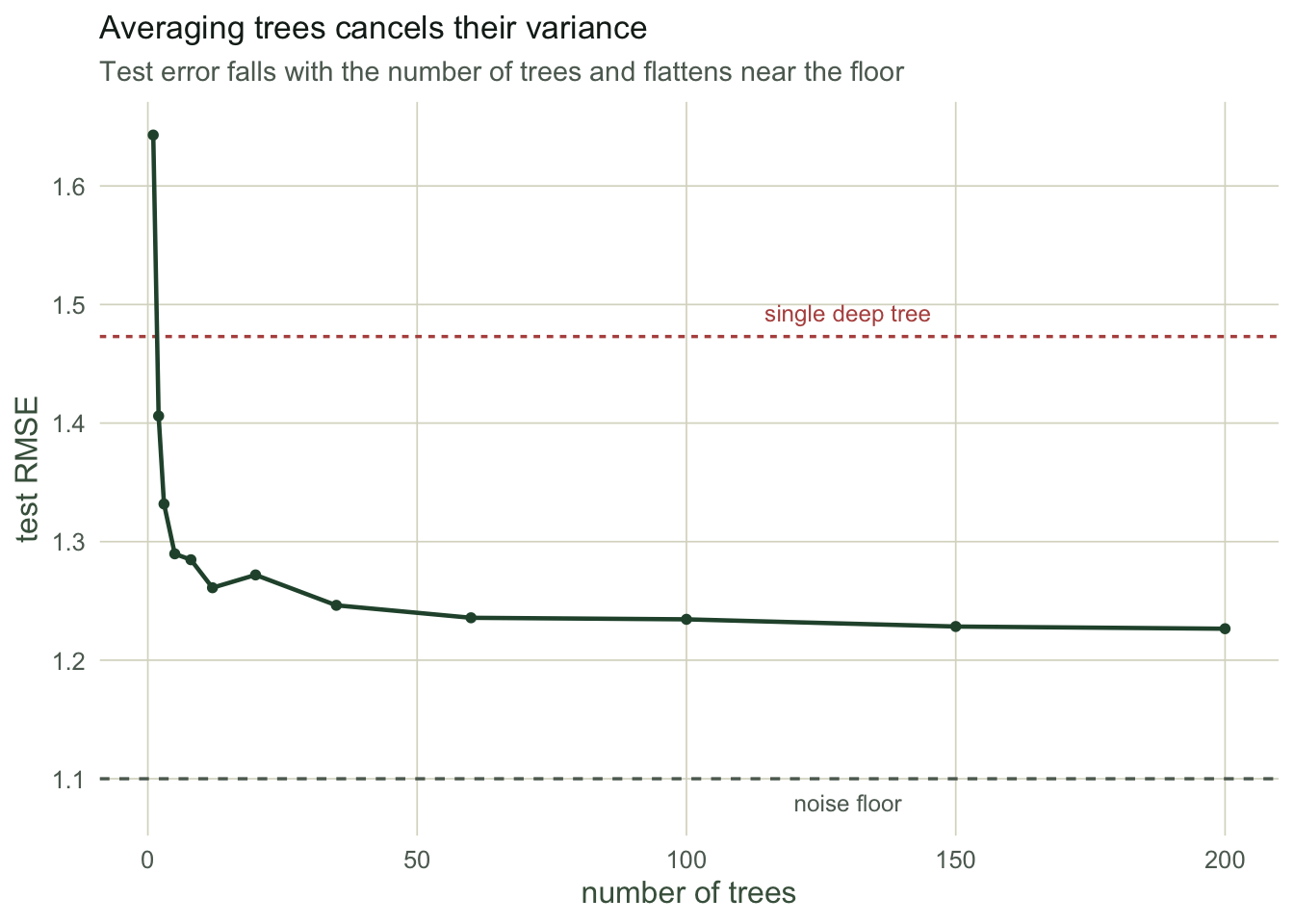
A single deep tree has a test error of 1.473, well above the noise floor of 1.1, because it is fitting the sampling noise. Averaging 200 bagged trees drops the test error to 1.202, most of the way to the floor. The random forest sits at 1.227. The averaging is doing the heavy lifting: a pile of high-variance trees, each individually mediocre, combine into a low-variance predictor, because their errors partly cancel.

Test error of the random forest as trees are added. One tree is noisy; the error falls quickly and flattens near the noise floor. A single deep tree and the floor are shown for reference.

The out-of-bag error is free

Each bootstrap resample leaves out about a third of the plots, the out-of-bag sample for that tree. Predicting each plot using only the trees that did not see it gives an honest estimate of test error, with no separate holdout set spent. This is one of the quietly useful features of bagging.

oob_rmse <- function(ens){
  n <- nrow(X); S <- numeric(n); C <- numeric(n)
  for (b in seq_along(ens$trees)){ ix <- ens$oob[[b]]; if (!length(ix)) next
    S[ix] <- S[ix] + pred1(ens$trees[[b]], X[ix,,drop=FALSE]); C[ix] <- C[ix] + 1 }
  k <- C > 0; sqrt(mean((S[k]/C[k] - yv[k])^2))
}
bag_oob <- round(oob_rmse(bag), 3); rf_oob <- round(oob_rmse(rf), 3)

The out-of-bag error is 1.105 for bagging and 1.13 for the random forest, both close to the independent test errors of 1.202 and 1.227. It is a little optimistic here, as out-of-bag error can be, but it lands in the right place and it costs nothing. When data are scarce this is often how a tree ensemble is tuned and reported.

What mtry actually buys

Bagged trees are grown on similar data with all predictors available, so when one predictor dominates they tend to make the same splits and their errors are correlated. Correlated errors do not cancel as well when averaged. The mtry restriction breaks this: by hiding some predictors at each split, it forces different trees to use different variables, so the trees disagree more and their errors cancel more. We can measure the disagreement directly as the average correlation between individual tree predictions.

avg_tree_cor <- function(Pm, m = 40){ s <- Pm[,1:m]; C <- cor(s); mean(C[upper.tri(C)]) }
cor_bag <- round(avg_tree_cor(Pbag), 3); cor_rf <- round(avg_tree_cor(Prf), 3)

The average pairwise tree correlation is 0.833 for bagging and 0.731 for the random forest: the forest’s trees are meaningfully less alike, which is exactly the point of mtry. Whether that lower correlation also lowers the test error depends on the problem. Here it does not: bagging and the forest end up neck and neck, because our response leans heavily on one dominant predictor, and forcing trees to ignore it at some splits costs about as much accuracy as the decorrelation gains. The random forest’s edge is largest when several correlated predictors each carry signal, so that a tree denied one still has a useful substitute. And mtry is a knob, not a guarantee: the sensible default for regression, one third of the predictors, is a starting point to tune, not a law.

Which predictors matter: permutation importance

An ensemble is a black box in a way a single tree is not, so we need a summary of what it is using. The cleanest one is permutation importance: shuffle a predictor’s values in the out-of-bag data, see how much worse the out-of-bag prediction gets, and read the increase as the importance of that predictor. A predictor the forest relies on will hurt when scrambled; a predictor it ignores will not.

perm_imp <- function(ens){
  n <- nrow(X)
  score <- function(perm = NULL){
    S <- numeric(n); C <- numeric(n)
    for (b in seq_along(ens$trees)){ ix <- ens$oob[[b]]; if (!length(ix)) next
      M <- X[ix,,drop=FALSE]; if (!is.null(perm)) M[,perm] <- X[sample(ix), perm]
      S[ix] <- S[ix] + pred1(ens$trees[[b]], M); C[ix] <- C[ix] + 1 }
    k <- C > 0; sqrt(mean((S[k]/C[k] - yv[k])^2))
  }
  b0 <- score(); set.seed(3)
  sapply(1:8, function(j) score(j) - b0)
}
imp <- perm_imp(rf); names(imp) <- paste0("x",1:8)
imp_x1 <- round(imp["x1"],3); imp_x4 <- round(imp["x4"],3)

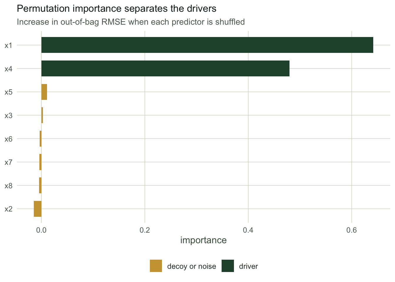
Temperature (x1) and moisture (x4), the two real drivers, rise clearly above the rest, at 0.642 and 0.479. The predictors correlated with them but with no direct effect (x2, x3, x5) sit near zero, and so do the pure-noise predictors. Permutation importance handles the correlated decoys well here, because the forest reaches for the true driver first and rarely needs its correlates, so shuffling them does little. That is the good news. The next post shows where variable importance stops being trustworthy, which is sooner than most write-ups admit.

Permutation importance from the random forest. The two real drivers stand out; the correlated decoys and the noise predictors sit near zero.

Where this leaves us

Bagging turns the unstable single tree into a stable predictor by averaging away its variance, and the out-of-bag error tells you how well it did without a holdout set. The random forest adds mtry to decorrelate the trees, which helps most when several predictors share the signal and can be a wash when one predictor dominates, as it was here. Both give a permutation-importance summary that, on this problem, correctly points at the two real drivers.

None of this makes the ensemble a smooth model or an explanatory one. It predicts, and it predicts well; it does not tell you the shape of the response or which predictor causes it. Boosting, the next post, takes a different route to a strong predictor: instead of averaging many independent trees, it grows small trees in sequence, each fixing the last one’s mistakes.

References

• Breiman 1996 Machine Learning 24(2):123-140 (10.1007/BF00058655).
• Breiman 2001 Machine Learning 45(1):5-32 (10.1023/A:1010933404324).
• Cutler, Edwards, Beard, Cutler, Hess, Gibson, Lawler 2007 Ecology 88(11):2783-2792 (10.1890/07-0539.1).
• Prasad, Iverson, Liaw 2006 Ecosystems 9(2):181-199 (10.1007/s10021-005-0054-1).
• Hastie, Tibshirani, Friedman 2009 The Elements of Statistical Learning (2nd ed), ISBN 978-0-387-84857-0.

Related tutorials

• Regression trees and CART
• Boosted regression trees
• Checking a tree ensemble
• Cross-validation and elastic net