library(rpart)
library(ggplot2)

## house theme
te_ink<-"#16241d"; te_body<-"#2c3a31"; te_forest<-"#275139"; te_label<-"#46604a"
te_paper<-"#f5f4ee"; te_line<-"#dad9ca"; te_faint<-"#5d6b61"
te_gold<-"#cda23f"; te_green<-"#2f8f63"; te_red<-"#b5534e"; te_lowc<-"#c9b458"; te_highc<-"#1d5b4e"
theme_te<-function(base_size=12){
  theme_minimal(base_size=base_size)+
  theme(text=element_text(colour=te_body),
    plot.title=element_text(colour=te_ink,size=rel(1.05)),
    plot.subtitle=element_text(colour=te_faint,size=rel(0.9)),
    axis.title=element_text(colour=te_label), axis.text=element_text(colour=te_faint),
    panel.grid.major=element_line(colour=te_line,linewidth=0.3), panel.grid.minor=element_blank(),
    plot.background=element_rect(fill="#f5f4ee",colour=NA), panel.background=element_rect(fill="#f5f4ee",colour=NA),
    legend.position="bottom", strip.text=element_text(colour=te_ink))
}

set.seed(4310)
n <- 240
x1 <- runif(n, 0, 10)   # temperature
x2 <- runif(n, 0, 10)   # moisture
f  <- ifelse(x1 < 5, 2 + 0.9*x2, 11 - 0.8*x2) + 1.2*(x1 > 7)*(x2 > 6)
sigma <- 2.0
y  <- f + rnorm(n, 0, sigma)
dat <- data.frame(y, x1, x2, f)

set.seed(99); tr <- sample(n, 160); te <- setdiff(1:n, tr)
rmse <- function(a, b) sqrt(mean((a - b)^2))Regression trees and CART, by hand
R
regression
machine learning
ecology tutorial
How a regression tree splits, why the greedy tree is unstable and overfits, and how cost-complexity pruning by cross-validation trades bias against variance.
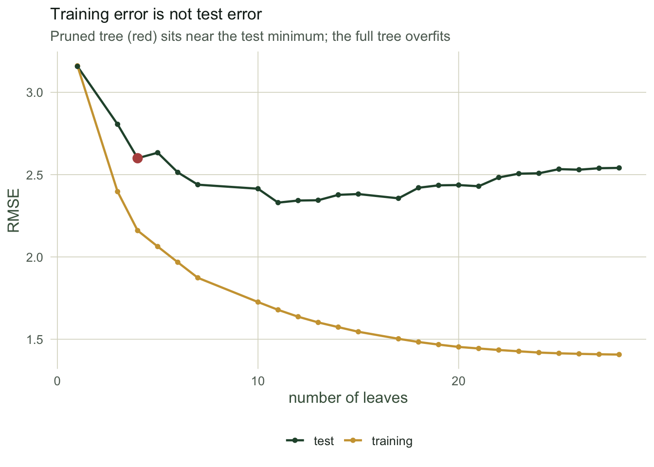
Corrected 27 September 2026: the caption of the error-curve figure said the one-standard-error rule picks a tree near the test-error minimum; it now says that on this test set somewhat larger trees do a little better, as the figure shows.
Most ecological models we have built here are additive and smooth: a linear predictor, a spline, a penalised fit. A regression tree throws that away and does something blunt instead. It cuts the predictor space into rectangular boxes with a sequence of yes/no questions, and predicts the mean of the response inside each box. The appeal is that it captures thresholds and interactions automatically, with no functional form to specify. The cost, which this post is really about, is that the tree is greedy, unstable, and happy to overfit.
We will grow a tree by hand so that the mechanics are not a black box, check it against rpart, and then meet the two problems that motivate everything in the rest of this cluster.
A regime-structured problem
The response is a biomass proxy on 240 plots, driven by temperature and moisture. Below a temperature threshold, biomass rises with moisture; above it, biomass falls with moisture (drought stress), with a bonus in the warm and wet corner. A tree should handle this regime switch cleanly, because that is exactly what axis-aligned splits are good at.
Growing a tree by hand
A regression tree is greedy. At every node it looks at each predictor, tries every possible split point, and keeps the single split that reduces the within-node sum of squares the most. Then it recurses on the two children. There is no look-ahead: a split that looks best now is taken even if a different first split would have led to a better tree overall.
sse <- function(v) if (length(v) == 0) 0 else sum((v - mean(v))^2)

best_split <- function(d, minbucket = 10) {
  base <- sse(d$y); best <- NULL; bestgain <- 0
  for (v in c("x1", "x2")) {
    xs <- d[[v]]; cand <- sort(unique(xs)); cand <- (head(cand, -1) + tail(cand, -1)) / 2
    for (s in cand) {
      L <- d$y[xs <= s]; R <- d$y[xs > s]
      if (length(L) < minbucket || length(R) < minbucket) next
      gain <- base - sse(L) - sse(R)
      if (gain > bestgain) { bestgain <- gain; best <- list(var = v, split = s, gain = gain) }
    }
  }
  best
}

grow <- function(d, depth = 0, maxdepth = 3, minsplit = 20, minbucket = 10) {
  if (nrow(d) < minsplit || depth >= maxdepth) return(list(leaf = TRUE, pred = mean(d$y)))
  bs <- best_split(d, minbucket)
  if (is.null(bs)) return(list(leaf = TRUE, pred = mean(d$y)))
  idx <- d[[bs$var]] <= bs$split
  list(leaf = FALSE, var = bs$var, split = bs$split, gain = bs$gain,
       left = grow(d[idx, , drop = FALSE], depth + 1, maxdepth, minsplit, minbucket),
       right = grow(d[!idx, , drop = FALSE], depth + 1, maxdepth, minsplit, minbucket))
}
predict_tree <- function(node, nd) {
  out <- numeric(nrow(nd))
  for (i in seq_len(nrow(nd))) { nn <- node
    while (!nn$leaf) nn <- if (nd[[nn$var]][i] <= nn$split) nn$left else nn$right
    out[i] <- nn$pred }
  out
}

ht <- grow(dat, maxdepth = 3)
root_var  <- ht$var
root_split<- round(ht$split, 3)
root_gain <- round(ht$gain, 1)
deep      <- round(c(ht$left$left$split, ht$left$right$split), 2)   # two levels below the root
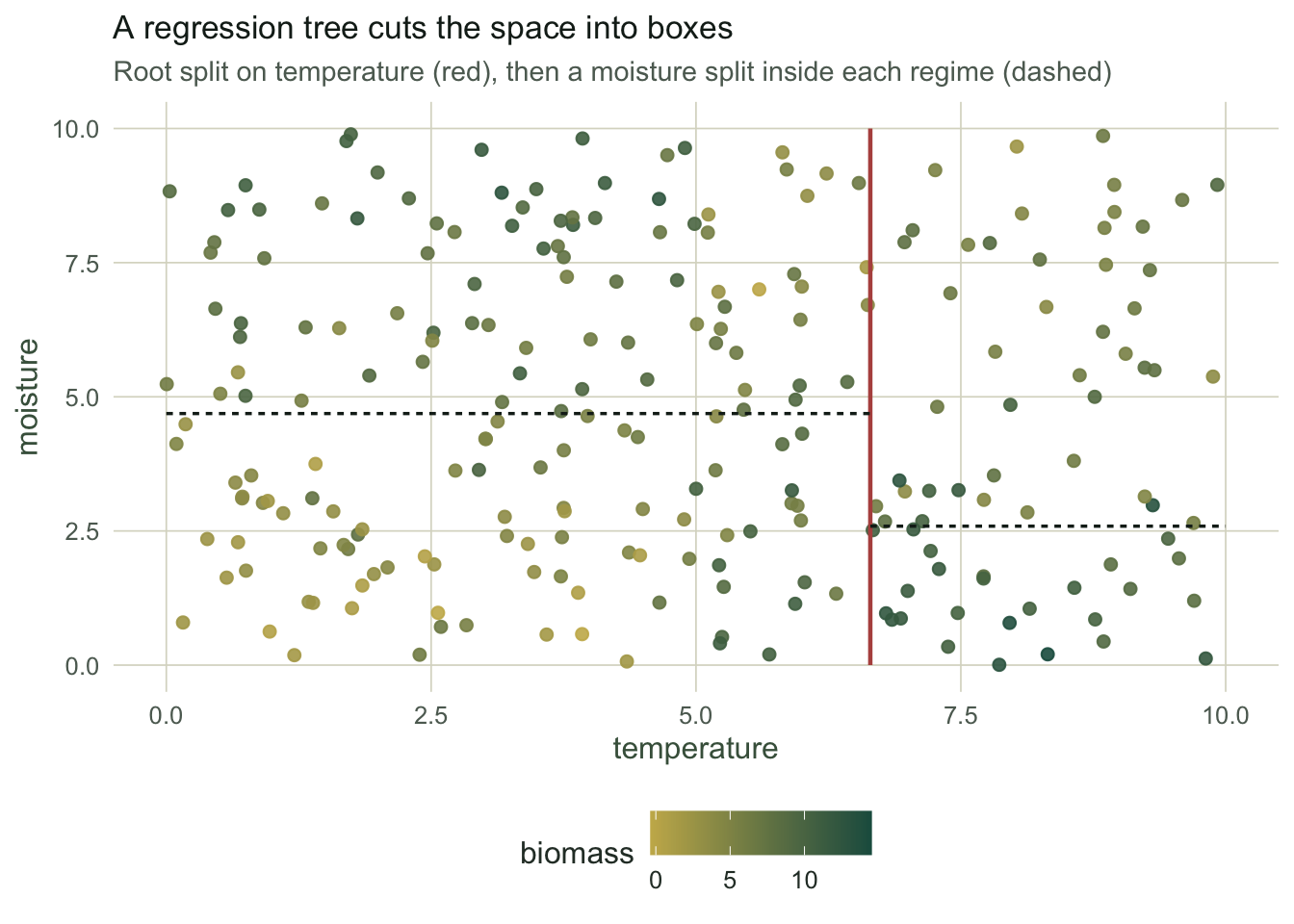
The first split is on x1 at 6.645, and it removes 204.4 units of sum of squares. Compare that number with the rule that generated the data, where the regime switches at a temperature of 5. The greedy search does not recover the boundary: it takes the cut that buys the most sum of squares immediately. The two second-level splits fall on moisture, one inside each side of the root, which is the interaction made visible. The generating threshold only shows up two levels down, as a pair of temperature splits at 4.97 and 5 inside the cool branch.
The point of coding this from scratch is to check it against the standard tool. Fitting rpart with the same depth and node-size limits gives the same tree:
rp <- rpart(y ~ x1 + x2, data = dat, method = "anova",
            control = rpart.control(maxdepth = 3, minsplit = 20, minbucket = 10, cp = 0, xval = 0))
rp_root_split <- round(rp$splits[1, "index"], 3)
max_diff <- signif(max(abs(predict_tree(ht, dat) - predict(rp, dat))), 3)
n_leaves <- length(unique(round(predict_tree(ht, dat), 6)))
rpart splits the root at 6.645, identical to the hand-grown value, and the fitted values agree to within floating-point rounding. Both trees have 8 leaves at depth three. The recursion is the whole algorithm.
Greedy trees overfit
Nothing in the growing rule tells the tree when to stop. Left alone it keeps splitting until the leaves are nearly pure, memorising the noise. The classic way to see this is to hold out a test set and grow three trees: a stump (one split), a fully grown tree, and a tree pruned back by cross-validation.
stump  <- rpart(y ~ x1 + x2, data = dat[tr, ], method = "anova",
                control = rpart.control(maxdepth = 1, xval = 0))
full   <- rpart(y ~ x1 + x2, data = dat[tr, ], method = "anova",
                control = rpart.control(cp = 0, minsplit = 4, minbucket = 2, xval = 0))
set.seed(2020)
grid   <- rpart(y ~ x1 + x2, data = dat[tr, ], method = "anova",
                control = rpart.control(cp = 0, minsplit = 10, minbucket = 5, xval = 10))
cpt <- grid$cptable
im  <- which.min(cpt[, "xerror"]); se <- cpt[im, "xerror"] + cpt[im, "xstd"]
i1  <- which(cpt[, "xerror"] <= se)[1]
pruned <- prune(grid, cp = cpt[i1, "CP"])

lv <- function(m) sum(m$frame$var == "<leaf>")
tr_full<-round(rmse(predict(full,dat[tr,]),dat$y[tr]),3);  te_full<-round(rmse(predict(full,dat[te,]),dat$y[te]),3)
tr_prun<-round(rmse(predict(pruned,dat[tr,]),dat$y[tr]),3); te_prun<-round(rmse(predict(pruned,dat[te,]),dat$y[te]),3)
te_stmp<-round(rmse(predict(stump,dat[te,]),dat$y[te]),3)
floor_rmse <- round(rmse(dat$f[te], dat$y[te]), 3)
nl_full <- lv(full); nl_prun <- lv(pruned)
The fully grown tree has 70 leaves and a training error of 0.913, far below the noise floor, but a test error of 2.66. That gap is the overfitting: the tree fits the training noise, which does not transfer. The stump underfits, with a test error of 3.068. The pruned tree, with only 4 leaves, matches the training set less closely (2.16) but generalises best of the three, with a test error of 2.6. The irreducible floor set by the noise is about 2.132, so even the pruned tree is not far from the best any model could do here.
The tree is unstable
There is a second problem, separate from overfitting and just as important. A regression tree is a high-variance estimator: a small change in the data can change which split is chosen first, and everything below inherits that change. Resampling the plots with replacement and refitting shows how fragile the structure is.
set.seed(717); B <- 500; roots <- character(B); rootpt <- numeric(B)
for (b in 1:B) {
  ib <- sample(n, n, replace = TRUE)
  rb <- rpart(y ~ x1 + x2, data = dat[ib, ], method = "anova",
              control = rpart.control(maxdepth = 3, minsplit = 20, minbucket = 10, cp = 0, xval = 0))
  roots[b] <- rownames(rb$splits)[1]; rootpt[b] <- rb$splits[1, "index"]
}
root_tab <- round(prop.table(table(roots)), 3)
pct_x1 <- unname(root_tab["x1"]) * 100
qx1 <- round(quantile(rootpt[roots == "x1"], c(.25, .5, .75)), 2)
The root variable is temperature in 86.8% of resamples and moisture in the rest, so the choice of variable is fairly stable here. The choice of split point is not: across the resamples that split on temperature, the boundary lands anywhere from 2.86 to 6.64 (interquartile range). A single tree reports one number for that boundary and hides all of this variability. On a harder problem the root variable itself flips from resample to resample, and two analysts with two samples draw two different trees. That instability is not a bug to be tuned away; it is intrinsic to a single greedy tree, and it is precisely what averaging many trees is designed to cancel.
Pruning: cost-complexity by cross-validation
We used pruning above without saying how it works. Growing a full tree and cutting back is more reliable than trying to stop early, because a weak split can sit above a strong one. Cost-complexity pruning adds a penalty proportional to the number of leaves and cross-validates the penalty.
set.seed(2020)
big <- rpart(y ~ x1 + x2, data = dat, method = "anova",
             control = rpart.control(cp = 0, minsplit = 10, minbucket = 5, xval = 10))
cp2 <- big$cptable
jmin <- which.min(cp2[, "xerror"])
j1se <- which(cp2[, "xerror"] <= cp2[jmin, "xerror"] + cp2[jmin, "xstd"])[1]
leaves_min <- cp2[jmin, "nsplit"] + 1
leaves_1se <- cp2[j1se, "nsplit"] + 1
leaves_full <- sum(big$frame$var == "<leaf>")
On the full data the unpruned tree has 36 leaves. Cross-validation puts the error minimum at 12 leaves, and the one-standard-error rule, which prefers the smallest tree within one standard error of that minimum, chooses 8 leaves. The one-standard-error rule is the honest default: it protects against the ragged, hard-to-reproduce splits at the bottom of the tree, the same splits that the bootstrap above showed to be unstable.
Where this leaves us
A single regression tree buys you automatic thresholds and interactions, and it costs you a step-function fit, high variance, and a strong pull toward overfitting. Pruning tames the overfitting; it does nothing for the variance. The response cannot be smooth, because the tree can only predict a constant inside each box. The two failures point to the same fix: if one tree is unstable, average many of them. That is bagging, and its refinement the random forest, which the next post builds from these same pieces.
Two cautions carry forward. The split points are properties of this particular sample, not fixed features of the world, so read a tree as a description of these data rather than a discovered structure. And a tree, like any predictor here, tells you where the response changes, not why: the variable at the root is the one that reduces error, which is not the same as the one that causes the response.
References
- Breiman, Friedman, Olshen, Stone 1984 Classification and Regression Trees, ISBN 978-0-412-04841-8.
- De’ath, Fabricius 2000 Ecology 81(11):3178-3192 (10.1890/0012-9658(2000)081[3178:CARTAP]2.0.CO;2).
- Hastie, Tibshirani, Friedman 2009 The Elements of Statistical Learning, 2nd edition, ISBN 978-0-387-84857-0.
- Therneau, Atkinson 2019 An Introduction to Recursive Partitioning Using the RPART Routines, rpart vignette.
- James, Witten, Hastie, Tibshirani 2013 An Introduction to Statistical Learning, ISBN 978-1-4614-7137-0.