Boosted regression trees, by hand

How gradient boosting builds a strong predictor from a sequence of tiny trees, why the learning rate and the number of trees trade off, and how boosting overfits if you let it, built from scratch in R.

Bagging and the random forest build a strong predictor by averaging many deep trees grown in parallel, each on its own resample. Boosting takes the opposite route. It grows tiny trees in sequence, each one fitting what the previous trees got wrong, and adds them up slowly. The result is often a slightly better predictor than a random forest, but it comes with a knob that bagging does not have: boosting will overfit if you add too many trees. We build it from scratch to see exactly why, and then look at how it is tuned in practice.

The idea: fit the residuals, slowly

Start with a constant prediction, the mean of the response. Look at the residuals, the part the current model gets wrong. Fit a small tree to those residuals, and add a shrunken version of it to the model. Now the residuals are a little smaller; repeat. Each tree is a small correction, and the learning rate controls how much of each correction you keep. For squared-error loss the residual is exactly the negative gradient of the loss, which is why this stagewise residual-fitting is called gradient boosting.

library(rpart); library(ggplot2)
te_ink<-"#16241d"; te_body<-"#2c3a31"; te_forest<-"#275139"; te_label<-"#46604a"
te_line<-"#dad9ca"; te_faint<-"#5d6b61"; te_gold<-"#cda23f"; te_red<-"#b5534e"; te_blue<-"#3f6f8f"
theme_te<-function(base_size=12){
  theme_minimal(base_size=base_size)+
  theme(text=element_text(colour=te_body),
    plot.title=element_text(colour=te_ink,size=rel(1.05)),
    plot.subtitle=element_text(colour=te_faint,size=rel(0.9)),
    axis.title=element_text(colour=te_label), axis.text=element_text(colour=te_faint),
    panel.grid.major=element_line(colour=te_line,linewidth=0.3), panel.grid.minor=element_blank(),
    plot.background=element_rect(fill="white",colour=NA), panel.background=element_rect(fill="white",colour=NA),
    legend.position="bottom", strip.text=element_text(colour=te_ink))
}
make_data <- function(n, seed){
  set.seed(seed)
  g1 <- rnorm(n); x1 <- g1+rnorm(n,0,0.6); x2 <- g1+rnorm(n,0,0.6); x3 <- g1+rnorm(n,0,0.6)
  g2 <- rnorm(n); x4 <- g2+rnorm(n,0,0.6); x5 <- g2+rnorm(n,0,0.6)
  x6 <- rnorm(n); x7 <- rnorm(n); x8 <- rnorm(n)
  f <- 2.2*(x1>0) + 0.9*x4 + 1.3*(x1>0)*(x4>0)
  data.frame(y = f + rnorm(n,0,1.1), x1,x2,x3,x4,x5,x6,x7,x8, f)
}
d  <- make_data(400, 511)
te <- make_data(4000, 999)
preds <- paste0("x",1:8); fo <- as.formula(paste("r ~", paste(preds, collapse=" + ")))
rmse <- function(a,b) sqrt(mean((a-b)^2)); floor_r <- round(rmse(te$f, te$y), 3)

The whole algorithm is a short loop. Each pass fits one small tree to the current residuals and updates the running prediction by a fraction of it.

boost <- function(dtr, M, lr, depth = 2){
  Fx <- rep(mean(dtr$y), nrow(dtr)); trees <- vector("list", M)
  for (m in 1:M){
    dd <- dtr; dd$r <- dtr$y - Fx                       # current residuals
    t <- rpart(fo, dd, method = "anova",
               control = rpart.control(maxdepth = depth, cp = 0, minsplit = 10, xval = 0, maxsurrogate = 0))
    trees[[m]] <- t; Fx <- Fx + lr * predict(t, dtr)    # add a shrunken correction
  }
  list(trees = trees, lr = lr, init = mean(dtr$y))
}
# fitted value after each successive tree, so we can read the error at any number of trees
fit_path <- function(bm, nd){
  Pm <- sapply(bm$trees, function(t) predict(t, nd))    # one column per tree
  bm$init + bm$lr * t(apply(Pm, 1, cumsum))             # column m = fit using the first m trees
}

The learning rate and the number of trees trade off

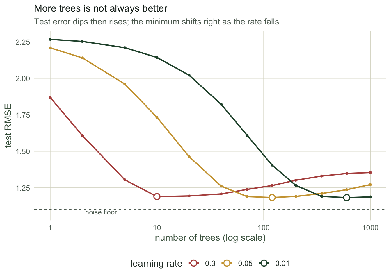
The learning rate and the number of trees are not independent choices. A large learning rate takes big steps and reaches a good fit in few trees, but it is coarse. A small learning rate takes tiny steps, needs many more trees to get there, and generally ends up a little better. We fit the same data at three learning rates and read off the test error as a function of the number of trees.

Ms <- c(1,2,5,10,20,40,70,120,200,350,600,1000)
curve_for <- function(lr){
  bm <- boost(d, max(Ms), lr, depth = 2)
  path <- fit_path(bm, te)
  te_err <- sapply(Ms, function(m) rmse(path[, m], te$y))
  data.frame(M = Ms, rmse = te_err, lr = factor(lr))
}
set.seed(1)
cv <- do.call(rbind, lapply(c(0.30, 0.05, 0.01), curve_for))
best <- do.call(rbind, lapply(split(cv, cv$lr), function(g) g[which.min(g$rmse), ]))
best_fast <- best[best$lr=="0.3",]; best_mid <- best[best$lr=="0.05",]; best_slow <- best[best$lr=="0.01",]

At a learning rate of 0.3 the best test error, 1.189, arrives after only 10 trees. At 0.05 the minimum is 1.183 at 120 trees, and at 0.01 it is 1.182 at 600 trees. Slower learning needs far more trees for the same job and edges out a slightly lower error, which is why the standard advice is to set the learning rate as low as your compute budget allows and then use as many trees as that rate needs. All three beat the random forest from the previous post, which sat at 1.226: fitting the residuals in sequence extracts a little more of the signal than averaging independent trees, and here the noise floor is 1.1.

Test error against the number of trees for three learning rates. Each curve dips to a minimum then rises: past the minimum, extra trees fit noise. Slower rates need more trees and overfit more gently.

Boosting will overfit if you let it

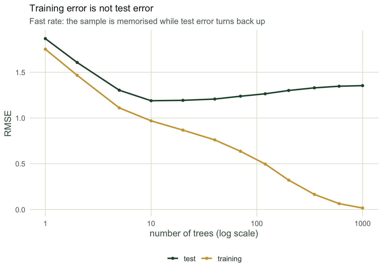
This is the part that separates boosting from bagging. Averaging trees cannot overfit by adding more of them: the random forest error flattened and stayed flat. Boosting keeps fitting residuals, so once it has captured the signal it starts fitting the noise, and the test error turns back up while the training error keeps falling towards zero. The gap between the two curves is the overfitting, laid bare.

bm_fast <- boost(d, 1000, lr = 0.30, depth = 2)
Mg <- c(1,2,5,10,20,40,70,120,200,350,600,1000)
path_tr <- fit_path(bm_fast, d); path_te <- fit_path(bm_fast, te)   # column m = fit using first m trees
of <- data.frame(M = rep(Mg, 2),
  rmse = c(sapply(Mg, function(m) rmse(path_tr[,m], d$y)),
           sapply(Mg, function(m) rmse(path_te[,m], te$y))),
  set = rep(c("training","test"), each = length(Mg)))
train_end <- round(rmse(path_tr[,1000], d$y), 3)   # after all 1000 trees
test_end  <- round(rmse(path_te[,1000], te$y), 3)

With the fast rate driven out to 1000 trees, the training error has fallen to 0.016, essentially memorising the sample, while the test error has climbed to 1.355, far worse than its own minimum. A model that fits the training data almost perfectly is not a triumph here; it is the warning sign.

Training and test error for a fast learning rate as trees accumulate. The training error falls towards zero while the test error passes a minimum and rises. Fitting the sample perfectly is overfitting, not success.

Tree depth sets the interaction order

The other lever is the size of each tree. A stump, one split, can only add up single-predictor effects; the ensemble it builds is purely additive and cannot represent an interaction no matter how many stumps you stack. Our response has a real interaction between the temperature threshold and moisture, so a depth-two learner, which can split twice, should beat a stump.

best_at <- function(depth){
  bm <- boost(d, 600, lr = 0.05, depth = depth)
  path <- fit_path(bm, te); min(sapply(c(50,100,200,350,600), function(m) rmse(path[,m], te$y)))
}
rmse_stump <- round(best_at(1), 3); rmse_depth2 <- round(best_at(2), 3)

The additive model of stumps bottoms out at 1.215, while the depth-two learner reaches 1.181. The difference is the interaction the stumps cannot see. Interaction depth is therefore a modelling choice, not a detail: it fixes the highest order of interaction the ensemble can represent, and like the learning rate and the tree count it is tuned, usually by cross-validation, not guessed.

Where this leaves us

Boosting is a strong and flexible predictor, and on this problem it beats both bagging and the random forest. That flexibility is also its hazard: three coupled knobs (the learning rate, the number of trees, and the interaction depth) all have to be set, the number of trees has a real optimum that more is not better than, and the training error is actively misleading because a well-boosted model can fit the sample almost perfectly while generalising worse. In ecology the standard recipe, from the boosted-regression-tree guides, is a slow learning rate, enough trees for that rate, a modest interaction depth, and the number of trees chosen by cross-validation with the training error ignored.

That covers building tree ensembles. The next and final post in this series is the one that matters most for using them in ecology: how to read what an ensemble tells you without fooling yourself. Variable importance, partial-dependence plots, and the out-of-bag error all have failure modes that are easy to walk into, and correlated predictors and spatial structure make them worse.

References

• Friedman 2001 Annals of Statistics 29(5):1189-1232 (10.1214/aos/1013203451).
• Elith, Leathwick, Hastie 2008 Journal of Animal Ecology 77(4):802-813 (10.1111/j.1365-2656.2008.01390.x).
• De’ath 2007 Ecology 88(1):243-251 (10.1890/0012-9658(2007)88[243:BTFEMA]2.0.CO;2).
• Hastie, Tibshirani, Friedman 2009 The Elements of Statistical Learning (2nd ed), ISBN 978-0-387-84857-0.

Related tutorials

• Bagging and random forests
• Regression trees and CART
• Checking a tree ensemble
• Cross-validation and elastic net