library(ggplot2)

te_pal <- list(forest = "#275139", green = "#2f8f63", sage = "#93a87f",
               clay = "#b5534e", gold = "#cda23f", line = "#dad9ca",
               ink = "#16241d", paper = "#f5f4ee")

theme_te <- function() {
  theme_minimal(base_size = 12) +
    theme(panel.grid.minor = element_blank(),
          panel.grid.major = element_line(colour = "#e7e6dc"),
          plot.background = element_rect(fill = "#f5f4ee", colour = NA),
          panel.background = element_rect(fill = "#f5f4ee", colour = NA),
          plot.title = element_text(face = "bold", colour = te_pal$ink),
          axis.title = element_text(colour = "#2c3a31"))
}Data leakage in ecological model validation
R
machine learning
model evaluation
model diagnostics
ecology tutorial
ggplot2
Four routes by which information crosses from a held-out fold into an ecological model fit, each measured in R: preprocessing, screening, grouped sites, tuning.
A model that scores well in cross-validation and then disappoints on the next field season is a common enough story to have stopped being interesting. What stays interesting is that the cross-validation was usually correct as arithmetic: folds were formed, each was held out in turn, predictions were made for rows the model had not seen. What went wrong happened earlier, in a line of code that ran before the folds existed.
Leakage is any path by which information about the held-out rows reaches the step being scored on them. The paths are mundane: you standardise a predictor, fill in a missing covariate, keep the twenty variables that correlate best with the response, try a few settings and report the best. Each is a decision taken with the whole dataset in view, and each leaves a fingerprint on the number you publish as an out-of-sample error.
The best-known route in ecology is spatial: sites near each other resemble each other, so a randomly chosen validation site usually has a training site a few hundred metres away, and the model is scored on an easier question than the one it will face. Spatial cross-validation for species distribution models measures that case, and this tutorial does not repeat it. What follows are the other routes, less discussed and, in one case, far worse.
Four of them, each simulated so the truth is known. Three are measured three ways: the error the leaky procedure reports, the error it reports once the leak is closed, and the error the fitted model makes on data that took no part in any of it. The screening route gets the first two only; its data hold no signal, so the leak-free cross-validation is the reference there. The last section ranks them by the gap my own runs produced.
Preprocessing computed on the whole dataset
Every preprocessing step belongs inside the training fold. The advice is correct, and for some steps it is also worth nothing, which is worth knowing: a rule that buys nothing gets dropped alongside the rules that matter.
The dataset is 120 sites with three covariates and a continuous response, the third missing at 35 per cent of sites, as happens when a soil sample is lost or a logger fails. Three preprocessing steps are compared, each run twice: once on the whole dataset before the folds are made, once refitted inside every training fold. The first centres and scales two complete covariates. The second fills the missing covariate with the overall mean of the observed values. The third fills it from a regression that includes the response, which the imputation literature recommends and which is sound for inference about coefficients, but which, run once on the whole dataset, puts each held-out site’s own response into that site’s covariate.
set.seed(20260815)
n_site <- 120
miss_frac <- 0.35
k_fold <- 10
n_rep1 <- 60
n_test <- 2000

sim_soil <- function(nn) {
  xa <- rnorm(nn)
  xb <- rnorm(nn)
  xc <- 0.5 * xa + rnorm(nn)
  yy <- 1.0 * xa + 0.4 * xb + 0.8 * xc + rnorm(nn, 0, 1)
  seen <- runif(nn) > miss_frac
  data.frame(xa = xa, xb = xb, xc = ifelse(seen, xc, NA_real_), y = yy)
}
rmse <- function(a, b) sqrt(mean((a - b)^2))
make_folds <- function(nn, kk) sample(rep(seq_len(kk), length.out = nn))

cv_standardise <- function(dd, fl, whole) {
  pred <- numeric(nrow(dd))
  if (whole) { mu <- c(mean(dd$xa), mean(dd$xb)); sg <- c(sd(dd$xa), sd(dd$xb)) }
  for (kk in unique(fl)) {
    tr <- dd[fl != kk, ]; va <- dd[fl == kk, ]
    if (!whole) { mu <- c(mean(tr$xa), mean(tr$xb)); sg <- c(sd(tr$xa), sd(tr$xb)) }
    trs <- data.frame(xa = (tr$xa - mu[1]) / sg[1], xb = (tr$xb - mu[2]) / sg[2], y = tr$y)
    vas <- data.frame(xa = (va$xa - mu[1]) / sg[1], xb = (va$xb - mu[2]) / sg[2])
    pred[fl == kk] <- predict(lm(y ~ xa + xb, data = trs), vas)
  }
  pred
}

cv_meanfill <- function(dd, fl, whole) {
  pred <- numeric(nrow(dd))
  gm <- mean(dd$xc, na.rm = TRUE)
  for (kk in unique(fl)) {
    tr <- dd[fl != kk, ]; va <- dd[fl == kk, ]
    fillv <- if (whole) gm else mean(tr$xc, na.rm = TRUE)
    tr$xc[is.na(tr$xc)] <- fillv; va$xc[is.na(va$xc)] <- fillv
    pred[fl == kk] <- predict(lm(y ~ xa + xb + xc, data = tr), va)
  }
  pred
}

cv_regfill <- function(dd, fl, whole) {
  pred <- numeric(nrow(dd))
  if (whole) {
    im <- lm(xc ~ xa + y, data = dd[!is.na(dd$xc), ])
    filled <- dd
    filled$xc[is.na(dd$xc)] <- predict(im, dd[is.na(dd$xc), ])
  }
  for (kk in unique(fl)) {
    if (whole) {
      tr <- filled[fl != kk, ]; va <- filled[fl == kk, ]
    } else {
      tr <- dd[fl != kk, ]; va <- dd[fl == kk, ]
      im <- lm(xc ~ xa, data = tr[!is.na(tr$xc), ])
      tr$xc[is.na(tr$xc)] <- predict(im, tr[is.na(tr$xc), ])
      va$xc[is.na(va$xc)] <- predict(im, va[is.na(va$xc), ])
    }
    pred[fl == kk] <- predict(lm(y ~ xa + xb + xc, data = tr), va)
  }
  pred
}

fresh_error <- function(dd, te, variant) {
  if (variant == "A") {
    mu <- c(mean(dd$xa), mean(dd$xb)); sg <- c(sd(dd$xa), sd(dd$xb))
    trs <- data.frame(xa = (dd$xa - mu[1]) / sg[1], xb = (dd$xb - mu[2]) / sg[2], y = dd$y)
    tes <- data.frame(xa = (te$xa - mu[1]) / sg[1], xb = (te$xb - mu[2]) / sg[2])
    return(rmse(predict(lm(y ~ xa + xb, data = trs), tes), te$y))
  }
  tr <- dd; va <- te
  if (variant == "B") {
    fillv <- mean(dd$xc, na.rm = TRUE)
    tr$xc[is.na(tr$xc)] <- fillv; va$xc[is.na(va$xc)] <- fillv
  } else {
    im <- lm(xc ~ xa, data = tr[!is.na(tr$xc), ])
    tr$xc[is.na(tr$xc)] <- predict(im, tr[is.na(tr$xc), ])
    va$xc[is.na(va$xc)] <- predict(im, va[is.na(va$xc), ])
  }
  rmse(predict(lm(y ~ xa + xb + xc, data = tr), va), va$y)
}

acc1 <- matrix(0, n_rep1, 9)
gap_a <- 0
for (r in seq_len(n_rep1)) {
  dd <- sim_soil(n_site); te <- sim_soil(n_test)
  fl <- make_folds(n_site, k_fold)
  pw <- cv_standardise(dd, fl, TRUE); pf <- cv_standardise(dd, fl, FALSE)
  gap_a <- max(gap_a, max(abs(pw - pf)))
  acc1[r, ] <- c(rmse(pw, dd$y), rmse(pf, dd$y),
                 rmse(cv_meanfill(dd, fl, TRUE), dd$y), rmse(cv_meanfill(dd, fl, FALSE), dd$y),
                 rmse(cv_regfill(dd, fl, TRUE), dd$y), rmse(cv_regfill(dd, fl, FALSE), dd$y),
                 fresh_error(dd, te, "A"), fresh_error(dd, te, "B"), fresh_error(dd, te, "C"))
}
pm <- colMeans(acc1)
prep_res <- data.frame(
  step = c("centre and scale", "fill missing by mean", "fill missing using y"),
  leaky = pm[c(1, 3, 5)], leak_free = pm[c(2, 4, 6)], fresh = pm[c(7, 8, 9)])
prep_res$optimism <- 1 - prep_res$leaky / prep_res$fresh
cat(sprintf("replicates %d, sites %d, missing fraction %.2f, folds %d, fresh sites %d\n",
            n_rep1, n_site, miss_frac, k_fold, n_test))
replicates 60, sites 120, missing fraction 0.35, folds 10, fresh sites 2000print(round(prep_res[, -1], 4)) leaky leak_free fresh optimism
1 1.2922 1.2922 1.2931 0.0007
2 1.1401 1.1404 1.1384 -0.0015
3 0.9440 1.1236 1.1233 0.1596cat(sprintf("largest gap between the two standardised fold predictions: %.2e\n", gap_a))largest gap between the two standardised fold predictions: 5.33e-15cat(sprintf("mean-fill optimism in rmse units: %.5f\n", prep_res$leak_free[2] - prep_res$leaky[2]))mean-fill optimism in rmse units: 0.00026cat(sprintf("regression-fill optimism: %.4f rmse units, %.1f percent of the fresh-site error\n",
prep_res$fresh[3] - prep_res$leaky[3], 100 * prep_res$optimism[3]))regression-fill optimism: 0.1793 rmse units, 16.0 percent of the fresh-site errorRow one is a flat nothing. Standardising on the whole dataset gives a cross-validated error of 1.2922 and standardising inside each fold gives 1.2922, the largest difference between any pair of fold predictions across 60 replicate datasets being 5.33e-15: floating point noise. Least squares is invariant to a linear rescaling of a predictor, so the coefficient absorbs the change and the fitted values do not move, whoever’s mean was used. Fresh sites cost 1.2931.
Row two, the overall-mean fill, is almost as quiet: the leaky version comes in 0.00026 lower, a difference about as large as the ink used to print it. The mean runs over the sites whose value was observed, about 78 of the 120, so any one held-out site moves it only slightly, and a held-out site whose own value is missing, the only kind the fill touches, does not move it at all. Nor does the mean know anything about the response.
Row three is a different animal: 0.9440 against 1.1236 for the same procedure kept inside the folds, and 1.1233 on 2000 sites that took no part in anything. The reported error is 16.0 per cent below the truth, and the procedure that produced it cannot be run in the field at all, because at the moment of prediction there is no response to impute from.
scheme_lv <- c("leaky: all rows at once", "leak-free: inside each fold",
               "fresh sites")
prep_long <- data.frame(
  step = rep(prep_res$step, 3),
  scheme = rep(scheme_lv, each = 3),
  err = c(prep_res$leaky, prep_res$leak_free, prep_res$fresh))
prep_long$step <- factor(prep_long$step, levels = prep_res$step)
prep_long$scheme <- factor(prep_long$scheme, levels = scheme_lv)
p_prep <- ggplot(prep_long, aes(err, step, colour = scheme, shape = scheme)) +
  geom_point(size = 3.4, position = position_dodge(width = 0.55)) +
  scale_colour_manual(values = c(te_pal$clay, te_pal$forest, te_pal$gold)) +
  scale_shape_manual(values = c(16, 15, 17)) +
  labs(title = "Only the step that sees the response leaks",
       x = "root mean squared error", y = NULL, colour = NULL, shape = NULL) +
  theme_te() +
  theme(legend.position = "top")
print(p_prep)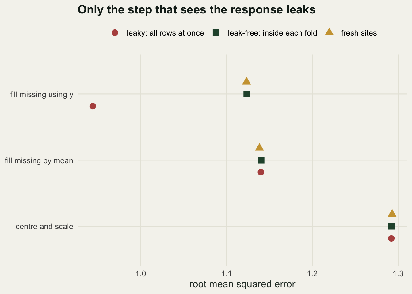
The dividing line is not before or after the folds were made. It is whether the step looked at the response. Centring, scaling, fixed log transforms and unsupervised imputation are functions of the predictors alone, and their leak is bounded by the influence of one held-out row on a summary of all rows. Anything that consults the response is a different case: response-guided imputation, dropping rows whose response looks extreme, encoding a factor by its mean response. Those belong inside the fold; the rest belong there for tidiness.
Screening predictors before the fold
Now the version that does real damage, on a dataset chosen so there is nothing to find. The response is standard normal noise, and so are the candidate predictors, independent of it and of each other. Sixty observations, a generous plot count for many field studies, and a number of candidates that sweeps from 40 up to 2560: the sort of range you get from a spectral library, a set of remote sensing bands and their ratios, or a table of metabarcoding counts.
The screen keeps the 8 predictors with the largest absolute correlation with the response. Run it once on the whole dataset, then cross-validate a linear model on the survivors, which is what happens when screening lives in a separate script from model fitting. Then run the same screen inside each training fold, where it sees only the rows the model sees.
set.seed(4711)
n_obs <- 60
n_keep <- 8
n_rep2 <- 30
p_grid <- c(40, 160, 640, 2560)

screen_top <- function(xx, yy, kk) order(abs(cor(xx, yy)), decreasing = TRUE)[seq_len(kk)]

cv_screen <- function(xx, yy, fl, inside, kk) {
  pred <- numeric(length(yy))
  if (!inside) sel_all <- screen_top(xx, yy, kk)
  for (ff in unique(fl)) {
    tr <- fl != ff
    sel <- if (inside) screen_top(xx[tr, , drop = FALSE], yy[tr], kk) else sel_all
    dtr <- data.frame(y = yy[tr], xx[tr, sel, drop = FALSE])
    dva <- data.frame(xx[!tr, sel, drop = FALSE])
    colnames(dtr) <- c("y", paste0("v", seq_len(kk)))
    colnames(dva) <- paste0("v", seq_len(kk))
    pred[!tr] <- predict(lm(y ~ ., data = dtr), dva)
  }
  1 - sum((yy - pred)^2) / sum((yy - mean(yy))^2)
}

screen_res <- data.frame(candidates = p_grid, leaky = 0, leak_free = 0)
for (i in seq_along(p_grid)) {
  pp <- p_grid[i]
  acc2 <- matrix(0, n_rep2, 2)
  for (r in seq_len(n_rep2)) {
    xx <- matrix(rnorm(n_obs * pp), n_obs, pp)
    yy <- rnorm(n_obs)
    fl <- make_folds(n_obs, k_fold)
    acc2[r, ] <- c(cv_screen(xx, yy, fl, FALSE, n_keep), cv_screen(xx, yy, fl, TRUE, n_keep))
  }
  screen_res[i, 2:3] <- colMeans(acc2)
}
cat(sprintf("observations %d, predictors kept %d, folds %d, replicates %d, true R-squared %d\n",
            n_obs, n_keep, k_fold, n_rep2, 0))
observations 60, predictors kept 8, folds 10, replicates 30, true R-squared 0print(round(screen_res, 4)) candidates leaky leak_free
1 40 0.0840 -0.2952
2 160 0.2469 -0.4008
3 640 0.4011 -0.3346
4 2560 0.4713 -0.4179cat(sprintf("at %d candidates: leaky cross-validated R-squared %.4f, leak-free %.4f\n",
p_grid[4], screen_res$leaky[4], screen_res$leak_free[4]))at 2560 candidates: leaky cross-validated R-squared 0.4713, leak-free -0.4179cat(sprintf("rmse ratio at %d candidates: %.4f\n", p_grid[4],
sqrt((1 - screen_res$leaky[4]) / (1 - screen_res$leak_free[4]))))rmse ratio at 2560 candidates: 0.6106With 40 candidates the cross-validated R-squared is 0.0840, which a cautious reader might wave away as a weak result. With 640 it is 0.4011. With 2560 it is 0.4713, on data in which no predictor has any relationship with the response, from a cross-validation that held out every row in turn and never fitted a model to a row it scored.
screen_long <- data.frame(
  candidates = rep(screen_res$candidates, 2),
  scheme = rep(c("screened on the whole dataset", "screened inside each fold"), each = 4),
  r2 = c(screen_res$leaky, screen_res$leak_free))
p_screen <- ggplot(screen_long, aes(candidates, r2, colour = scheme)) +
  geom_hline(yintercept = 0, linetype = "dashed", colour = te_pal$ink) +
  geom_line(linewidth = 0.9) +
  geom_point(size = 2.6) +
  scale_x_log10(breaks = p_grid) +
  scale_colour_manual(values = c(te_pal$forest, te_pal$clay)) +
  labs(title = "Cross-validated fit to data that contains no signal",
       x = "candidate predictors offered to the screen (log scale)",
       y = "cross-validated R-squared", colour = NULL) +
  theme_te() +
  theme(legend.position = "top")
print(p_screen)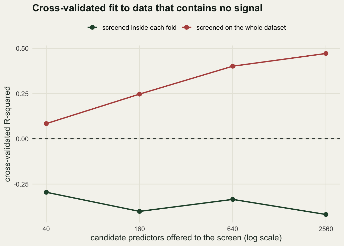
Move the screen inside the fold and the whole thing collapses. At 2560 candidates the cross-validated R-squared is -0.4179, and the honest answer is not zero. Zero is what predicting the mean would give; the leak-free procedure still fits 8 arbitrary predictors to 54 training rows and pays for them, so it lands below the mean. That is the correct verdict on a model built this way, and a leak-free cross-validation delivers it plainly. In error units the leaky estimate is 0.6106 times the honest one.
The mechanism is not subtle once you see it. The screen sifts 2560 columns of noise for the handful that happen to correlate with the response in these particular 60 rows, and those correlations are accidents of the response values, including the values in every future validation fold. By the time the folds are made, the columns already know the answer.
This is the one to worry about, because the leak is invisible where anyone looks for it: the model fitting is clean, the folds are clean, and the damage was done in a preceding script. It also has no ceiling, since offering more candidates keeps the reported fit climbing.
Folds that cut through a group
Ecological data are almost never one row per independent unit. Sites are revisited, colonies give up several individuals, plots hold several quadrats, stations run for several years. The rows within a group share whatever the group has that the covariates do not describe.
The simulation is 30 sites with 8 visits each, one covariate that varies visit to visit, and a site-level effect whose share of the total variance is the intraclass correlation. The model is a common slope plus a per-site intercept, which is what a fixed site term or a random intercept amounts to when the site has already been met; for a site the model has never met, the intercept falls back on the average. Random 10-fold cross-validation on rows is compared with leaving one whole site out, and both against the truth: fitting on all 240 rows and predicting 30 sites that were never in the data.
set.seed(90210)
n_grp <- 30
n_visit <- 8
n_rep3 <- 40
icc_grid <- c(0, 0.2, 0.4, 0.6, 0.8)

sim_grouped <- function(ng, nv, icc) {
  sd_b <- sqrt(icc); sd_e <- sqrt(1 - icc)
  gid <- rep(seq_len(ng), each = nv)
  bb <- rnorm(ng, 0, sd_b)
  xx <- rnorm(ng * nv)
  data.frame(site = gid, x = xx, y = 0.7 * xx + bb[gid] + rnorm(ng * nv, 0, sd_e))
}
fit_sites <- function(dd) {
  mm <- lm(y ~ x, data = dd)
  list(cf = coef(mm), off = tapply(residuals(mm), dd$site, mean))
}
pred_sites <- function(fitobj, nd) {
  oo <- fitobj$off[as.character(nd$site)]
  fitobj$cf[1] + fitobj$cf[2] * nd$x + ifelse(is.na(oo), 0, oo)
}
cv_rows <- function(dd, kk) {
  fl <- make_folds(nrow(dd), kk)
  pr <- numeric(nrow(dd))
  for (ff in unique(fl)) pr[fl == ff] <- pred_sites(fit_sites(dd[fl != ff, ]), dd[fl == ff, ])
  rmse(pr, dd$y)
}
cv_sites <- function(dd) {
  pr <- numeric(nrow(dd))
  for (gg in unique(dd$site))
    pr[dd$site == gg] <- pred_sites(fit_sites(dd[dd$site != gg, ]), dd[dd$site == gg, ])
  rmse(pr, dd$y)
}

grp_res <- data.frame(icc = icc_grid, random_k = 0, one_site_out = 0, new_sites = 0)
for (i in seq_along(icc_grid)) {
  acc3 <- matrix(0, n_rep3, 3)
  for (r in seq_len(n_rep3)) {
    dd <- sim_grouped(n_grp, n_visit, icc_grid[i])
    nw <- sim_grouped(n_grp, n_visit, icc_grid[i])
    nw$site <- nw$site + n_grp * 100
    acc3[r, ] <- c(cv_rows(dd, k_fold), cv_sites(dd),
                   rmse(pred_sites(fit_sites(dd), nw), nw$y))
  }
  grp_res[i, 2:4] <- colMeans(acc3)
}
grp_res$ratio <- grp_res$one_site_out / grp_res$random_k
grp_res$predicted <- 1 / (sqrt(1 - icc_grid) * sqrt(1 + 1 / (n_visit - 1)))
cat(sprintf("sites %d, visits per site %d, rows %d, replicates %d, total variance %d\n",
            n_grp, n_visit, n_grp * n_visit, n_rep3, 1))
sites 30, visits per site 8, rows 240, replicates 40, total variance 1print(round(grp_res, 4)) icc random_k one_site_out new_sites ratio predicted
1 0.0 1.0647 0.9859 1.0241 0.9259 0.9354
2 0.2 0.9666 1.0114 1.0186 1.0464 1.0458
3 0.4 0.8434 1.0156 1.0096 1.2042 1.2076
4 0.6 0.6749 0.9919 1.0237 1.4697 1.4790
5 0.8 0.4872 1.0386 1.0346 2.1319 2.0917cat(sprintf("at icc %.1f: random %d-fold %.4f against new sites %.4f, optimism %.1f percent\n",
icc_grid[5], k_fold, grp_res$random_k[5], grp_res$new_sites[5],
100 * (1 - grp_res$random_k[5] / grp_res$new_sites[5])))at icc 0.8: random 10-fold 0.4872 against new sites 1.0346, optimism 52.9 percentcat(sprintf("at icc %.1f: random %d-fold %.4f, one-site-out %.4f, new sites %.4f\n",
icc_grid[1], k_fold, grp_res$random_k[1], grp_res$one_site_out[1],
grp_res$new_sites[1]))at icc 0.0: random 10-fold 1.0647, one-site-out 0.9859, new sites 1.0241cat(sprintf("no-site-effect inflation sqrt(1 + 1/(visits - 1)) = %.4f\n",
sqrt(1 + 1 / (n_visit - 1))))no-site-effect inflation sqrt(1 + 1/(visits - 1)) = 1.0690grp_long <- data.frame(
icc = rep(grp_res$icc, 3),
scheme = rep(c("random 10-fold on rows", "leave one site out", "fresh sites"), each = 5),
err = c(grp_res$random_k, grp_res$one_site_out, grp_res$new_sites))
p_grp <- ggplot(grp_long, aes(icc, err, colour = scheme, linetype = scheme)) +
geom_line(linewidth = 0.9) +
geom_point(size = 2.6) +
scale_colour_manual(values = c(te_pal$gold, te_pal$forest, te_pal$clay)) +
scale_linetype_manual(values = c("dashed", "solid", "solid")) +
labs(title = "Random folds answer a question about sites you already visited",
x = "intraclass correlation of the site effect",
y = "root mean squared error", colour = NULL, linetype = NULL) +
theme_te() +
theme(legend.position = "top")
print(p_grp)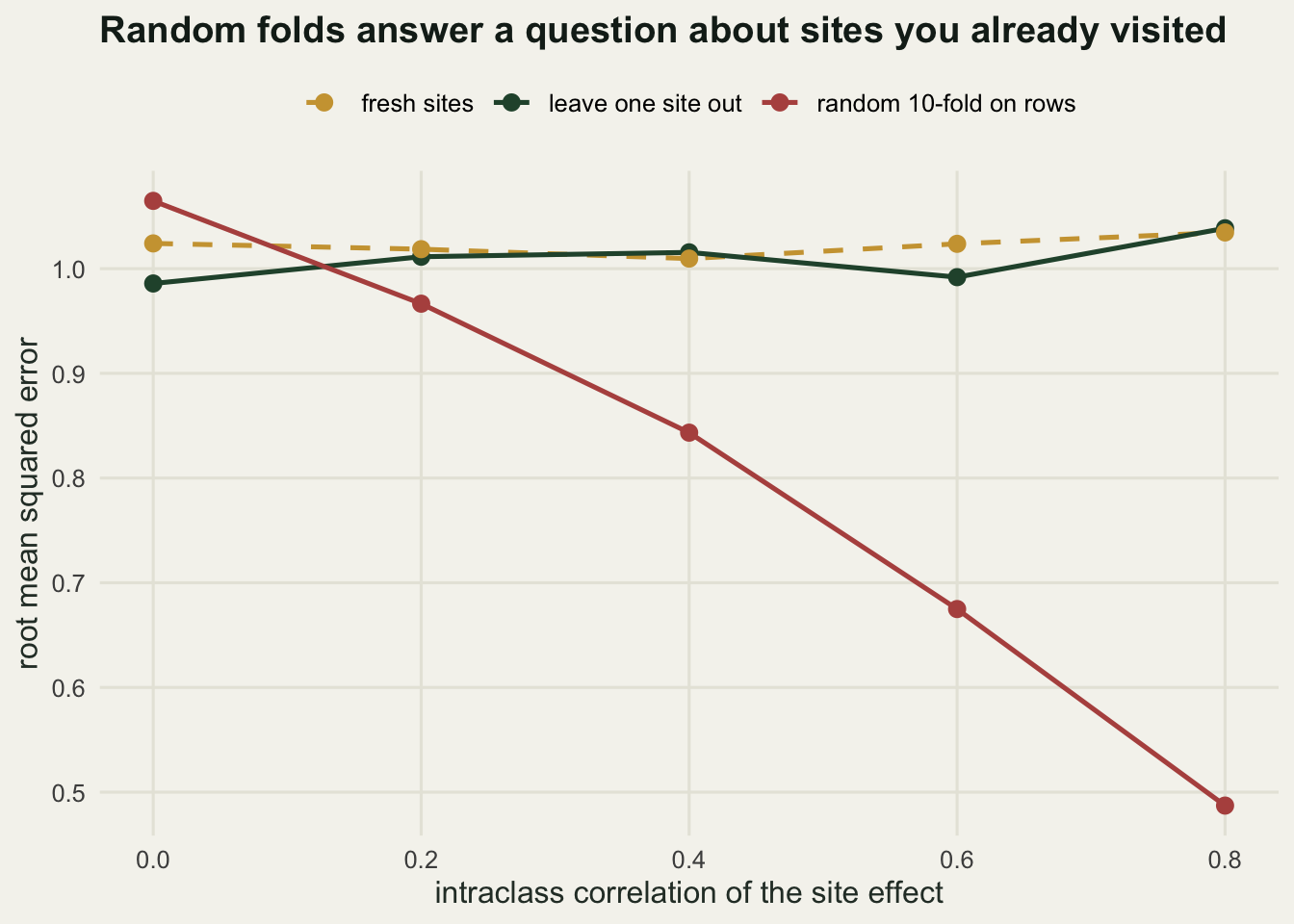
At an intraclass correlation of 0.8, random 10-fold cross-validation reports 0.4872 while the same model costs 1.0346 on sites it has never visited: 52.9 per cent too low. Leaving one site out gives 1.0386, right to within its own noise. The ratio between the two schemes is 2.1319 there, against 2.0917 from the closed form 1 / (sqrt(1 - icc) * sqrt(1 + 1 / (visits - 1))), and the agreement holds down the whole column. Random folds are not a worse estimate of the same quantity. They estimate a different one: the error of predicting a new visit to a site you have already characterised.
Sometimes that is the question: if the model will be applied to the same long-term plots forever, random folds answer it. Usually it is not, because the sentence in the discussion says the model can be applied to unsurveyed sites.
The first row goes the other way. With no site effect at all, random 10-fold gives 1.0647 and leaving a site out gives 0.9859, so the leaky scheme is pessimistic: the per-site intercepts are then pure noise estimated from 7 other visits, and carrying them costs a measured factor of 1.0800, against the 1.0690 that sqrt(1 + 1/(visits - 1)) predicts. A leak needs something to leak.
Choosing the model on the folds you report
The fourth route is the most respectable-looking. You have a tuning decision, so you cross-validate across the candidates, take the best, and report its cross-validated error as the performance of the model. Nothing was fitted to held-out rows at any point. The leak is in the selection: the reported number is a minimum over many noisy estimates, and a minimum over noise is biased downwards.
The setting is 50 rows and 20 predictors, of which 4 carry an effect. The tuning decision is which candidate covariate subset to use, each a random draw of 5 predictors, which is what trying a pile of plausible formulations looks like written down honestly. The sweep runs from one candidate, where there is no selection, up to 100. The flat estimate is the best cross-validated error over those tried; nested cross-validation repeats the whole search inside each outer training set, and the truth is 3000 fresh rows.
set.seed(1848)
n_tr <- 50
n_pred <- 20
n_sub <- 5
k_out <- 5
k_in <- 5
n_cand <- 100
n_rep4 <- 60
n_big <- 3000
g_grid <- c(1, 3, 10, 30, 100)
b_true <- c(0.6, -0.5, 0.4, 0.3, rep(0, 16))

sim_tune <- function(nn) {
  xx <- matrix(rnorm(nn * n_pred), nn, n_pred)
  list(x = xx, y = as.vector(xx %*% b_true) + rnorm(nn, 0, 1.2))
}
cv_cands <- function(xx, yy, cands, kk) {
  fl <- make_folds(length(yy), kk)
  sse <- numeric(length(cands))
  for (ff in unique(fl)) {
    tr <- which(fl != ff); va <- which(fl == ff)
    for (j in seq_along(cands)) {
      sel <- cands[[j]]
      cf <- .lm.fit(cbind(1, xx[tr, sel, drop = FALSE]), yy[tr])$coefficients
      sse[j] <- sse[j] + sum((yy[va] - cbind(1, xx[va, sel, drop = FALSE]) %*% cf)^2)
    }
  }
  sse / length(yy)
}
refit_pred <- function(xtr, ytr, xte, sel) {
  cf <- .lm.fit(cbind(1, xtr[, sel, drop = FALSE]), ytr)$coefficients
  as.vector(cbind(1, xte[, sel, drop = FALSE]) %*% cf)
}

acc4 <- array(0, c(n_rep4, length(g_grid), 3))
for (r in seq_len(n_rep4)) {
  dd <- sim_tune(n_tr); bg <- sim_tune(n_big)
  cands <- lapply(seq_len(n_cand), function(i) sample(n_pred, n_sub))
  flat_curve <- cv_cands(dd$x, dd$y, cands, k_out)
  fl <- make_folds(n_tr, k_out)
  sse_nest <- numeric(length(g_grid))
  for (ff in unique(fl)) {
    tr <- which(fl != ff); va <- which(fl == ff)
    inner <- cv_cands(dd$x[tr, ], dd$y[tr], cands, k_in)
    for (i in seq_along(g_grid)) {
      jj <- which.min(inner[seq_len(g_grid[i])])
      pr <- refit_pred(dd$x[tr, ], dd$y[tr], dd$x[va, ], cands[[jj]])
      sse_nest[i] <- sse_nest[i] + sum((dd$y[va] - pr)^2)
    }
  }
  for (i in seq_along(g_grid)) {
    jb <- which.min(flat_curve[seq_len(g_grid[i])])
    pr <- refit_pred(dd$x, dd$y, bg$x, cands[[jb]])
    acc4[r, i, ] <- c(flat_curve[jb], sse_nest[i] / n_tr, mean((bg$y - pr)^2))
  }
}
tune_res <- data.frame(tried = g_grid, flat = apply(acc4[, , 1], 2, mean),
                       nested = apply(acc4[, , 2], 2, mean),
                       fresh = apply(acc4[, , 3], 2, mean))
tune_res$optimism <- 1 - tune_res$flat / tune_res$fresh
cat(sprintf("rows %d, predictors %d, subset size %d, outer %d, inner %d, replicates %d, fresh rows %d\n",
            n_tr, n_pred, n_sub, k_out, k_in, n_rep4, n_big))
rows 50, predictors 20, subset size 5, outer 5, inner 5, replicates 60, fresh rows 3000cat(sprintf("noise variance %.2f\n", 1.2^2))noise variance 1.44print(round(tune_res, 4)) tried flat nested fresh optimism
1 1 2.3974 2.3681 2.3728 -0.0103
2 3 2.1625 2.4297 2.3449 0.0778
3 10 1.9275 2.4094 2.2604 0.1473
4 30 1.7544 2.3059 2.1906 0.1991
5 100 1.6609 2.2872 2.0933 0.2066cat(sprintf("with %d candidates: flat %.4f, nested %.4f, fresh %.4f, optimism %.1f percent\n",
g_grid[5], tune_res$flat[5], tune_res$nested[5], tune_res$fresh[5],
100 * tune_res$optimism[5]))with 100 candidates: flat 1.6609, nested 2.2872, fresh 2.0933, optimism 20.7 percentcat(sprintf("rmse ratio at %d candidates: %.4f\n", g_grid[5],
sqrt(tune_res$flat[5] / tune_res$fresh[5])))rmse ratio at 100 candidates: 0.8908tune_long <- data.frame(
tried = rep(tune_res$tried, 3),
scheme = rep(c("reported: best flat cross-validated error", "nested cross-validation",
"fresh rows"), each = 5),
err = c(tune_res$flat, tune_res$nested, tune_res$fresh))
p_tune <- ggplot(tune_long, aes(tried, err, colour = scheme, linetype = scheme)) +
geom_line(linewidth = 0.9) +
geom_point(size = 2.6) +
scale_x_log10(breaks = g_grid) +
scale_colour_manual(values = c(te_pal$gold, te_pal$forest, te_pal$clay)) +
scale_linetype_manual(values = c("dashed", "solid", "solid")) +
labs(title = "The winner's curse grows with the size of the search",
x = "candidate configurations tried (log scale)",
y = "mean squared error", colour = NULL, linetype = NULL) +
theme_te() +
theme(legend.position = "top")
print(p_tune)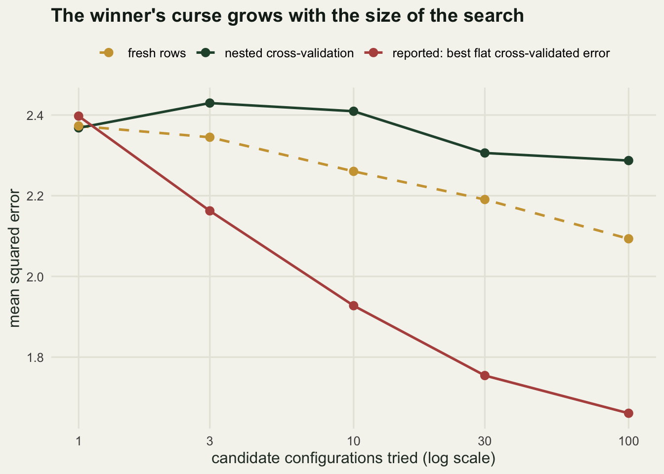
With one candidate there is no selection and the flat estimate behaves: 2.3974 reported against 2.3728 on fresh rows. With 100 candidates the reported error is 1.6609 and the fresh rows cost 2.0933, an optimism of 20.7 per cent in squared error and a factor of 0.8908 in error units. The search does something real as well, since the fresh-row error improves too: a search over 100 subsets finds subsets that hold the predictors that matter. Both are true at once, and only one appears in the reported number.
Nested cross-validation tracks the truth: 2.2872 against 2.0933 at the widest search. It errs on the pessimistic side, and it should, because every outer training set is 40 rows rather than 50 and a smaller training set makes a worse model. That is the standing objection to it, and it is the right direction to be wrong in.
The phrase “the bias grows with the size of the search” then needs a qualification. Tune a ridge penalty instead, on the same datasets, with either 4 penalties spanning the grid or all 100.
set.seed(31337)
n_rep5 <- 120
lam_all <- 10^seq(-1, 2.5, length.out = 100)
idx_four <- unique(round(seq(1, length(lam_all), length.out = 4)))

ridge_all <- function(xx, yy, lams) {
  mx <- colMeans(xx); my <- mean(yy)
  xc <- sweep(xx, 2, mx)
  sv <- svd(xc)
  uy <- as.vector(crossprod(sv$u, yy - my))
  list(b = sv$v %*% ((sv$d * uy) / outer(sv$d^2, lams, "+")), mx = mx, my = my)
}
ridge_pred <- function(fitobj, xx) fitobj$my + sweep(xx, 2, fitobj$mx) %*% fitobj$b
ridge_curve <- function(xx, yy, lams, kk) {
  fl <- make_folds(length(yy), kk)
  sse <- numeric(length(lams))
  for (ff in unique(fl)) {
    tr <- fl != ff
    fitobj <- ridge_all(xx[tr, , drop = FALSE], yy[tr], lams)
    sse <- sse + colSums((yy[!tr] - ridge_pred(fitobj, xx[!tr, , drop = FALSE]))^2)
  }
  sse / length(yy)
}

acc5 <- matrix(0, n_rep5, 4)
for (r in seq_len(n_rep5)) {
  dd <- sim_tune(n_tr); bg <- sim_tune(n_big)
  cc <- ridge_curve(dd$x, dd$y, lam_all, k_out)
  fitobj <- ridge_all(dd$x, dd$y, lam_all)
  pt <- ridge_pred(fitobj, bg$x)
  j_all <- which.min(cc)
  j_four <- idx_four[which.min(cc[idx_four])]
  acc5[r, ] <- c(cc[j_four], mean((bg$y - pt[, j_four])^2),
                 cc[j_all], mean((bg$y - pt[, j_all])^2))
}
rm5 <- colMeans(acc5)
cat(sprintf("ridge penalties on the same %d datasets, %d predictors, %d rows\n",
            n_rep5, n_pred, n_tr))
ridge penalties on the same 120 datasets, 20 predictors, 50 rowscat(sprintf("4 penalties: flat %.4f, fresh %.4f, optimism %.1f percent\n",
rm5[1], rm5[2], 100 * (1 - rm5[1] / rm5[2])))4 penalties: flat 1.9318, fresh 1.9641, optimism 1.6 percentcat(sprintf("%d penalties: flat %.4f, fresh %.4f, optimism %.1f percent\n",
length(lam_all), rm5[3], rm5[4], 100 * (1 - rm5[3] / rm5[4])))100 penalties: flat 1.8967, fresh 1.9537, optimism 2.9 percentFour penalties give an optimism of 1.6 per cent and 100 penalties give 2.9 per cent. Widening that search by a factor of twenty-five barely moves it, where the comparable step in the subset search, from 3 candidates to 100, moved the optimism from 7.8 per cent to 20.7 per cent. The count of candidates is not what matters. What matters is how different they are: neighbouring penalties on a smooth grid give nearly the same predictions and nearly the same cross-validation error, so there is little independent noise for the minimum to exploit. A hundred distinct covariate sets are a hundred separate lottery tickets.
Ranking the four routes
Each route was measured on its own scale, so the table below puts them on one: reported error divided by honest error, both as root mean squared error, so that 1 means no leak and 0.5 means the reported error is half of what the model will deliver. Honest error means the fresh-data error on every row but the screening one, whose data contain no signal; there the leak-free cross-validation stands in.
rank_res <- data.frame(
  route = c("screening on the whole dataset", "random folds on grouped rows",
            "imputation that uses the response", "tuning on the folds you report",
            "penalty grid tuned on the folds you report", "mean fill on the whole dataset",
            "centre and scale on the whole dataset"),
  dial = c("2560 candidate predictors", "icc 0.8", "35 percent missing",
           "100 configurations", "100 penalties", "35 percent missing", "none"),
  reported_over_honest = c(
    sqrt((1 - screen_res$leaky[4]) / (1 - screen_res$leak_free[4])),
    grp_res$random_k[5] / grp_res$new_sites[5],
    prep_res$leaky[3] / prep_res$fresh[3],
    sqrt(tune_res$flat[5] / tune_res$fresh[5]),
    sqrt(rm5[3] / rm5[4]),
    prep_res$leaky[2] / prep_res$fresh[2],
    prep_res$leaky[1] / prep_res$fresh[1]))
rank_res$optimism_pct <- 100 * (1 - rank_res$reported_over_honest)
rank_res <- rank_res[order(-rank_res$optimism_pct), ]
row.names(rank_res) <- NULL
print(rank_res, digits = 3)
route dial
1 random folds on grouped rows icc 0.8
2 screening on the whole dataset 2560 candidate predictors
3 imputation that uses the response 35 percent missing
4 tuning on the folds you report 100 configurations
5 penalty grid tuned on the folds you report 100 penalties
6 centre and scale on the whole dataset none
7 mean fill on the whole dataset 35 percent missing
reported_over_honest optimism_pct
1 0.471 52.9132
2 0.611 38.9369
3 0.840 15.9628
4 0.891 10.9249
5 0.985 1.4700
6 0.999 0.0712
7 1.001 -0.1472cat(sprintf("moderate settings: screening at %d candidates %.1f percent, grouping at icc %.1f %.1f percent\n",
p_grid[2], 100 * (1 - sqrt((1 - screen_res$leaky[2]) / (1 - screen_res$leak_free[2]))),
icc_grid[3], 100 * (1 - grp_res$random_k[3] / grp_res$new_sites[3])))moderate settings: screening at 160 candidates 26.7 percent, grouping at icc 0.4 16.5 percentAt the settings I ran, grouped rows split across random folds top the list at 52.9 per cent, predictor screening outside the folds follows at 38.9 per cent, response-aware imputation sits at 16.0 per cent, and tuning on the reported folds at 10.9 per cent. The two unsupervised preprocessing steps come out at 0.0712 per cent and -0.1472 per cent, which is zero with sampling noise on it.
That ordering is an artefact of where I set each dial, and the dials are not comparable. The grouping leak is capped by what the intraclass correlation allows: at 0.4, ordinary for repeated visits, it is 16.5 per cent. The screening leak has no cap. At 160 candidates it is already 26.7 per cent, and it climbs with every column you offer it.
Frequency and severity do not line up in any tidy way: the route that tops the list here is also the most common one. Grouped rows are nearly universal in field data, and the fix is the one people forget, because a group column looks like an ordinary column. Tuning on the reported folds is common wherever a model is picked by trying several versions and keeping the best, and it is the smallest of the four; the ridge grid measured earlier is milder still. Screening thousands of candidates is the rarest, confined to spectral, genomic and remote sensing data, which is where it does the most damage.
What a leak-free number still cannot tell you
Close every leak above and the cross-validated error estimates one thing: the error on new data drawn from the same distribution as the data you have. That is not usually the question. The question is a new region, a new decade, a different observer, different instruments.
The measurement below fits a linear model where the truth is mildly curved, then scores it two ways: on fresh data from the same distribution, and on data whose predictor mean has moved by 1.8 standard deviations, as it does when a model built in one region is applied in another.
set.seed(606)
n_lim <- 250
n_rep6 <- 150
shift_sd <- 1.8
sim_shift <- function(nn, mu) {
  xx <- rnorm(nn, mu, 1)
  data.frame(x = xx, y = 1.2 * xx + 0.5 * xx^2 + rnorm(nn, 0, 1))
}
acc6 <- matrix(0, n_rep6, 3)
for (r in seq_len(n_rep6)) {
  dd <- sim_shift(n_lim, 0)
  fl <- make_folds(n_lim, k_fold)
  pr <- numeric(n_lim)
  for (ff in unique(fl)) pr[fl == ff] <- predict(lm(y ~ x, data = dd[fl != ff, ]), dd[fl == ff, ])
  mm <- lm(y ~ x, data = dd)
  same <- sim_shift(n_test, 0)
  away <- sim_shift(n_test, shift_sd)
  acc6[r, ] <- c(rmse(pr, dd$y), rmse(predict(mm, same), same$y),
                 rmse(predict(mm, away), away$y))
}
lm6 <- colMeans(acc6)
cat(sprintf("rows %d, replicates %d, shift %.1f sd, fresh rows %d\n",
            n_lim, n_rep6, shift_sd, n_test))
rows 250, replicates 150, shift 1.8 sd, fresh rows 2000cat(sprintf("leak-free 10-fold %.4f, same distribution %.4f, shifted region %.4f, ratio %.2f\n",
lm6[1], lm6[2], lm6[3], lm6[3] / lm6[1]))leak-free 10-fold 1.2340, same distribution 1.2348, shifted region 2.7158, ratio 2.20The leak-free cross-validation gives 1.2340 and fresh data from the same distribution gives 1.2348, so the cross-validation did its job exactly. The same model, applied where the predictor mean has shifted, gives 2.7158, a factor of 2.20 worse. No arrangement of the folds could have revealed that. The curvature responsible is present in the 250 training rows, where a residual plot is the place to look for it, but folds cut from those rows cannot estimate an error in a region the rows do not reach.
So the honest cross-validated number is an upper bound on what a transfer will deliver, not an estimate of it. If the model is going somewhere new, the only measurement that answers the question is data from the new place. Blocking the folds by region or by year gets closer, because it forces some extrapolation, but a block that is still inside the same data cannot represent a place the data never visited.
Where to go next
A leak-free error estimate is a number about accuracy, and accuracy is not a decision. The last tutorial in this cluster, Choosing a decision threshold from costs, takes the step from a validated model to an action: where to put the cut-off when a missed occurrence and a wasted visit cost different amounts, and how far the answer moves when the cost ratio is known only to within a factor of two.
References
Ambroise C, McLachlan GJ 2002 Proceedings of the National Academy of Sciences 99(10):6562-6566 (10.1073/pnas.102102699)
Varma S, Simon R 2006 BMC Bioinformatics 7:91 (10.1186/1471-2105-7-91)
Roberts DR, Bahn V, Ciuti S, Boyce MS, Elith J, Guillera-Arroita G, Hauenstein S, Lahoz-Monfort JJ, Schroder B, Thuiller W, Warton DI, Wintle BA, Hartig F, Dormann CF 2017 Ecography 40(8):913-929 (10.1111/ecog.02881)
Kaufman S, Rosset S, Perlich C, Stitelman O 2012 ACM Transactions on Knowledge Discovery from Data 6(4):15 (10.1145/2382577.2382579)
Wenger SJ, Olden JD 2012 Methods in Ecology and Evolution 3(2):260-267 (10.1111/j.2041-210X.2011.00170.x)