library(ggplot2)
library(patchwork)

te_paper  <- "#f5f4ee"
te_ink    <- "#16241d"
te_body   <- "#2c3a31"
te_forest <- "#275139"
te_rust   <- "#b5534e"
te_gold   <- "#c9b458"
te_line   <- "#dad9ca"
te_sage   <- "#8aa37f"

theme_datasheet <- function() {
  theme_minimal(base_size = 12) +
    theme(plot.background  = element_rect(fill = te_paper, colour = NA),
          panel.background = element_rect(fill = te_paper, colour = NA),
          panel.grid.major = element_line(colour = te_line, linewidth = 0.3),
          panel.grid.minor = element_blank(),
          text             = element_text(colour = te_body),
          plot.title       = element_text(colour = te_ink, face = "bold"),
          plot.subtitle    = element_text(colour = te_body),
          axis.text        = element_text(colour = te_body))
}Leave-one-out AUC on a small survey
R
model evaluation
cross-validation
species distributions
simulation
ecology tutorial
Pooled leave-one-out AUC marks a working species model down on a small presence-absence survey. Measuring the bias in R, and why leave-pair-out avoids it.
Thirty ponds surveyed once for a scarce newt, and the newt found in nine of them. A logistic regression on one habitat score fits, the slope points the right way, and before anyone uses the model it has to be validated. There is no second survey to test it on, so the analyst does what small-sample advice recommends: leave each pond out in turn, refit on the other twenty-nine, predict the pond that was left out, then put the thirty held-out predictions together and compute one AUC. The number comes back lower than hoped, and a model that was doing its job gets described as weak.
On this site the pooling step already appears once, and there it is harmless. The post on spatial cross-validation for SDMs trains on four folds, predicts the fifth, and says in so many words that it then pools all held-out predictions and computes a single AUC. It does that on 1500 sites with 485 occupied, where one site’s label barely moves the refit. On a survey of thirty ponds with nine presences the same pooling ranks every held-out pond with a model refitted against it, and a working model is marked down by close to a tenth on the AUC scale before anyone has looked at it.
This is a known result, and the post demonstrates it rather than discovering it. Parker, Gunter and Bedo 2007 showed that pooled leave-one-out AUC falls well below one half on data with no signal at all, and called it stratification bias. Airola and colleagues 2011 compared cross-validation schemes for the AUC and found that leave-pair-out, which holds out one presence and one absence together and asks only whether that pair is ordered correctly, is close to unbiased. What is measured here is the size of the bias in the setting an ecologist actually meets, how it changes with the number of sites when the model has signal and when it has none, which part of the refit carries it, and what happens once the model has more than one covariate.
The direction is what separates it from the other validation numbers on this site. Every leak in data leakage in ecological model validation pushes a score up when there is something to leak, and the pessimistic numbers it does show come from elsewhere: nested cross-validation training on 40 rows rather than 50, and noise site intercepts carried by a random split when there is no site effect. Neither comes from the held-out label. In assignment tests and self-assignment leave-one-out is the repair for an upward bias. Here leave-one-out is the cause of a downward one, and it works through the held-out label itself. Evaluating species distribution models scores its model on a separate test set of 800 sites and never meets the problem.
Thirty ponds and one refit per pond
The generating model is a logistic regression with one standardised habitat covariate and an intercept set so that the expected share of occupied ponds is three in ten. The slope is fixed at 1.1, which gives a model whose AUC on new ponds is about three quarters: useful, not spectacular. A survey is redrawn if it has fewer than three presences or three absences, because the AUC is not defined without both.
# AUC as the share of presence-absence pairs ranked correctly (ties count one half)
auc_pairs <- function(score, y) {
  r <- rank(score); n1 <- sum(y == 1); n0 <- sum(y == 0)
  (sum(r[y == 1]) - n1 * (n1 + 1) / 2) / (n1 * n0)
}
fit_logit <- function(X, y, off = NULL)
  suppressWarnings(glm.fit(X, y, family = binomial(), offset = off)$coefficients)
# the criterion glm.fit uses for its "fitted probabilities numerically 0 or 1" warning
at_edge <- function(X, cf) {
  mu <- plogis(drop(X %*% cf)); e <- 10 * .Machine$double.eps
  any(mu < e | mu > 1 - e)
}

prev_set  <- 0.3      # expected share of occupied ponds
b_work    <- 1.1      # slope of the working model
min_class <- 3        # a survey needs at least three of each class
find_a <- function(b, prev)
  uniroot(function(a) mean(plogis(a + b * qnorm(ppoints(4000)))) - prev, c(-12, 5))$root

draw_survey <- function(n, b, prev, n_noise = 0) {
  a <- find_a(b, prev); p <- 1 + n_noise
  repeat {
    Z <- matrix(rnorm(n * p), n)
    y <- rbinom(n, 1, plogis(a + b * Z[, 1]))
    if (sum(y) >= min_class && sum(1 - y) >= min_class) break
  }
  list(X = cbind(1, Z), y = y, a = a, b = b, p = p)
}
Here is one survey, fitted to all thirty ponds and then refitted thirty times, once without each pond. For every pond the refit gives a held-out linear predictor, and the change from the full fit to the refit is the thing to look at.
set.seed(3030)
n_small <- 30
sv <- draw_survey(n_small, b_work, prev_set)
X <- sv$X; y <- sv$y
cf_full <- fit_logit(X, y)
eta_full <- drop(X %*% cf_full)
eta_loo <- vapply(seq_len(n_small), function(i)
  sum(X[i, ] * fit_logit(X[-i, , drop = FALSE], y[-i])), 0)
shift <- eta_loo - eta_full
n1_ex <- sum(y)
shift_pres <- mean(shift[y == 1]); shift_abs <- mean(shift[y == 0])
n_pres_down <- sum(shift[y == 1] < 0); n_abs_up <- sum(shift[y == 0] > 0); n0_ex <- sum(y == 0)
sd_eta_ex <- sd(eta_full); gap_ex <- median(diff(sort(eta_full)))
tilt_over_gap <- mean(abs(shift)) / gap_ex
pair_ok <- function(score) outer(score[y == 1], score[y == 0], ">")
n_flip <- sum(pair_ok(eta_full) & !pair_ok(eta_loo)); n_unflip <- sum(!pair_ok(eta_full) & pair_ok(eta_loo))
n_new <- 4000
Zn <- matrix(rnorm(n_new), n_new); yn <- rbinom(n_new, 1, plogis(sv$a + sv$b * Zn[, 1]))
truth_ex <- auc_pairs(cbind(1, Zn) %*% cf_full, yn)
auc_resub_ex <- auc_pairs(eta_full, y); auc_loo_ex <- auc_pairs(eta_loo, y)
This survey has 13 occupied ponds. Refitting without an occupied pond moves that pond’s own linear predictor by -0.194 on the logit scale on average, and refitting without an empty pond moves its own predictor by +0.127. The direction holds for 13 of the 13 presences and for 17 of the 17 absences. This survey happens to have a steep fit (a fitted slope of 3.92 against the true 1.1), with a standard deviation of 3.129 in the full-fit linear predictor across ponds, but the AUC is built from the gaps between neighbouring ponds, and the median gap is only 0.324. The average shift is 0.5 times that gap. In a survey with a fit this steep, 3 of the 197 presence-absence pairs that the full fit ordered correctly (out of 221) are put out of order by the refits, and 0 go the other way: the moves are few, and they all push in one direction.
The mechanism fits in two sentences. A model fitted without an occupied pond has seen one presence fewer, so it predicts occupancy a little lower everywhere and a little lower still near that pond’s covariate value; a model fitted without an empty pond does the reverse. Pooling then puts thirty predictions from thirty different models onto one ranking, and each pond is ranked by the model that was tilted against its own label.
The model fitted to all thirty ponds has a conditional AUC of 0.760 on 4000 fresh ponds drawn from the same process. That is the number the validation is trying to estimate. Resubstitution, scoring the thirty survey ponds with the full fit, gives 0.891, and pooled leave-one-out gives 0.878. Both sit above the truth because this particular survey orders its ponds unusually well, and the loss from pooling is a mild 0.014 here. One survey says little about an estimator; the sections below average over hundreds.
tilt_df <- data.frame(full = eta_full, loo = eta_loo,
                      status = factor(ifelse(y == 1, "occupied", "empty"),
                                      levels = c("occupied", "empty")))
tilt_df <- tilt_df[order(tilt_df$full), ]
tilt_df$pond <- seq_len(n_small)
ggplot(tilt_df, aes(y = pond, colour = status)) +
  geom_segment(aes(x = full, xend = loo, yend = pond), linewidth = 0.7,
               arrow = arrow(length = unit(0.12, "cm"), type = "closed")) +
  geom_point(aes(x = full), shape = 21, fill = te_paper, size = 2, stroke = 0.8) +
  scale_colour_manual(values = c(occupied = te_rust, empty = te_forest), name = NULL) +
  labs(x = "linear predictor (logit of occupancy)", y = "ponds, ordered by the full fit",
       title = "Each held-out pond is scored by a model tilted against it",
       subtitle = "occupied ponds move down, empty ponds move up") +
  theme_datasheet() + theme(legend.position = "bottom", axis.text.y = element_blank(),
                            panel.grid.major.y = element_blank())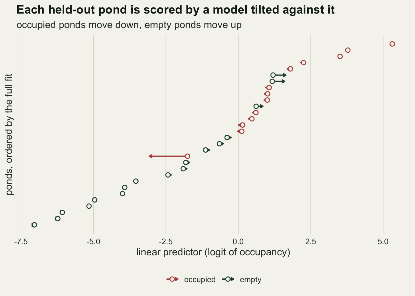
The limiting case shows the mechanism in its bare form. Drop the covariate and fit an intercept only. Leaving out an occupied pond then gives a held-out prediction equal to the occupied share among the other twenty-nine, which is one presence short, and leaving out an empty pond gives a share that is one presence long. Every held-out presence is scored below every held-out absence, and the pooled AUC is exactly zero.
X0 <- X[, 1, drop = FALSE]
loo_int <- vapply(seq_len(n_small), function(i) fit_logit(X0[-i, , drop = FALSE], y[-i]), 0)
auc_int <- auc_pairs(loo_int, y)
p_held_pres <- (n1_ex - 1) / (n_small - 1); p_held_abs <- n1_ex / (n_small - 1)
int_gap <- max(abs(plogis(loo_int) - ifelse(y == 1, p_held_pres, p_held_abs)))
On the example survey the refits give a pooled AUC of 0.0, with held-out probabilities of 0.4138 for every presence and 0.4483 for every absence, matching the fractions 12/29 and 13/29 to \(1.7 \times 10^{-10}\). That zero is arithmetic and serves only as an anchor. Everything from here on has a covariate in the model and is measured.
How far a working model is marked down
Six estimators are applied to the same simulated surveys. Resubstitution scores the survey with the model fitted to all of it. Pooled leave-one-out is the procedure from the opening. Pooled random five-fold and pooled stratified five-fold (each fold holding a fifth of the presences and a fifth of the absences) put all held-out predictions onto one ranking, as leave-one-out does. Per-fold stratified five-fold computes an AUC inside each held-out fold and averages the five. Leave-pair-out holds out one presence and one absence, refits on the rest, and scores whether the presence is ranked above the absence; averaged over pairs, that is the AUC.
The denominator matters, so here it is exactly. Every AUC below is the share of the presence-absence pairs in the survey that are ranked correctly by the held-out scores; for leave-pair-out it is the share of left-out pairs ranked correctly, over a random sample of 150 pairs per survey (a design constant, fixed in advance). The bias of an estimator is its value minus the conditional AUC of the model fitted to all ponds of that survey, computed on 4000 fresh ponds, taken per survey and then averaged over surveys.
n_pair <- 150
score_survey <- function(sv, n_pair = 150, n_new = 4000) {
  X <- sv$X; y <- sv$y; n <- length(y)
  cf_all <- fit_logit(X, y)
  Zn <- matrix(rnorm(n_new * sv$p), n_new)
  yn <- rbinom(n_new, 1, plogis(sv$a + sv$b * Zn[, 1]))
  truth <- auc_pairs(cbind(1, Zn) %*% cf_all, yn)
  e <- 10 * .Machine$double.eps
  loo_m <- vapply(seq_len(n), function(i) {
    cf <- fit_logit(X[-i, , drop = FALSE], y[-i])
    c(sum(X[i, ] * cf), at_edge(X[-i, , drop = FALSE], cf))
  }, numeric(2))
  # intercept held at its full-data value: only the slope is refitted
  slope_only <- if (sv$p == 1) auc_pairs(vapply(seq_len(n), function(i) {
    cf <- fit_logit(X[-i, 2, drop = FALSE], y[-i], off = rep(cf_all[1], n - 1))
    cf_all[1] + cf * X[i, 2] }, 0), y) else NA
  pooled_k <- function(folds) {
    s <- numeric(n)
    for (k in unique(folds)) {
      te <- folds == k
      s[te] <- X[te, , drop = FALSE] %*% fit_logit(X[!te, , drop = FALSE], y[!te])
    }
    s
  }
  f_rand <- sample(rep(1:5, length.out = n))
  f_str <- integer(n)
  f_str[y == 1] <- sample(rep(1:5, length.out = sum(y)))
  f_str[y == 0] <- sample(rep(1:5, length.out = sum(1 - y)))
  s_str <- pooled_k(f_str)
  per_fold <- vapply(1:5, function(k) {
    te <- f_str == k
    if (length(unique(y[te])) < 2) return(NA_real_)
    auc_pairs(s_str[te], y[te])
  }, 0)
  pairs <- as.matrix(expand.grid(which(y == 1), which(y == 0)))
  if (nrow(pairs) > n_pair) pairs <- pairs[sample(nrow(pairs), n_pair), ]
  lpo <- mean(apply(pairs, 1, function(ij) {
    cf <- fit_logit(X[-ij, , drop = FALSE], y[-ij])
    d <- sum((X[ij[1], ] - X[ij[2], ]) * cf)
    (d > 0) + 0.5 * (d == 0)
  }))
  c(truth = truth, resub = auc_pairs(X %*% cf_all, y), loo = auc_pairs(loo_m[1, ], y),
    rand5 = auc_pairs(pooled_k(f_rand), y), strat5 = auc_pairs(s_str, y),
    perfold = mean(per_fold, na.rm = TRUE), lpo = lpo, slope_only = slope_only,
    edge_full = at_edge(X, cf_all), edge_loo = mean(loo_m[2, ]),
    fold_na = sum(is.na(per_fold)), n1 = sum(y))
}

est_code <- c("resub", "loo", "rand5", "strat5", "perfold", "lpo")
est_lab  <- c("resubstitution", "pooled leave-one-out", "pooled random 5-fold",
              "pooled stratified 5-fold", "per-fold stratified 5-fold", "leave-pair-out")
est_col  <- setNames(c(te_gold, te_rust, te_rust, te_rust, te_forest, te_forest), est_lab)
batch_size <- 20
summarise_cell <- function(D, est = est_code) {
  B <- D[, est, drop = FALSE] - D[, "truth"]
  batch <- rep(seq_len(nrow(D) / batch_size), each = batch_size)
  bm <- apply(B, 2, function(v) tapply(v, batch, mean, na.rm = TRUE))
  data.frame(estimator = est, bias = colMeans(B, na.rm = TRUE),
             mcse = apply(B, 2, sd, na.rm = TRUE) / sqrt(colSums(!is.na(B))),
             rmse = sqrt(colMeans(B^2, na.rm = TRUE)),
             lo = apply(bm, 2, min), hi = apply(bm, 2, max),
             value = colMeans(D[, est, drop = FALSE], na.rm = TRUE))
}
run_cell <- function(n_ds, n, b, prev, n_noise = 0)
  t(replicate(n_ds, score_survey(draw_survey(n, b, prev, n_noise), n_pair)))
Four cells at thirty ponds: the working model, a weak model with the slope halved to 0.55, a null model with no slope at all, and the working model on a survey where the expected occupied share is one half rather than three in ten. Each cell gets 200 simulated surveys, run as batches of 20 so that the spread between batches can be shown alongside the Monte Carlo standard error.
n_ds_small <- 200
b_weak <- 0.55; b_null <- 0; prev_bal <- 0.5
small_spec <- data.frame(cell = c("working model", "weak model", "no signal", "balanced survey"),
                         b = c(b_work, b_weak, b_null, b_work),
                         prev = c(prev_set, prev_set, prev_set, prev_bal))
set.seed(4127)
t_small <- system.time(
  small_runs <- lapply(seq_len(nrow(small_spec)), function(k)
    run_cell(n_ds_small, n_small, small_spec$b[k], small_spec$prev[k])))
small_tab <- do.call(rbind, lapply(seq_len(nrow(small_spec)), function(k)
  cbind(cell = small_spec$cell[k], summarise_cell(small_runs[[k]]))))
small_tab$cell <- factor(small_tab$cell, levels = small_spec$cell)
small_tab$estimator <- factor(est_lab[match(small_tab$estimator, est_code)], levels = rev(est_lab))
cell_row <- function(cl, est) small_tab[small_tab$cell == cl & small_tab$estimator == est_lab[match(est, est_code)], ]
truth_mean <- vapply(small_runs, function(D) mean(D[, "truth"]), 0)
n1_mean <- mean(small_runs[[1]][, "n1"])
w_loo <- cell_row("working model", "loo"); w_lpo <- cell_row("working model", "lpo")
w_pf <- cell_row("working model", "perfold"); w_str <- cell_row("working model", "strat5")
w_rnd <- cell_row("working model", "rand5"); w_res <- cell_row("working model", "resub")
In the working model the conditional AUC averages 0.751 over the 200 surveys, which carry 9.1 presences on average. Pooled leave-one-out averages 0.660, a bias of -0.091 with a Monte Carlo standard error of 0.012; across the ten batches of twenty its batch means run from -0.139 to -0.034. That is the drop of close to a tenth promised in the opening. Pooled random five-fold is no better at -0.084, because it pools in the same way. Stratifying the folds removes part of it, leaving -0.040: stratification fixes the class balance of each fold but the pooled ranking still mixes five tilted models.
The two estimators that never compare predictions from different models do not show the bias. Per-fold averaging comes in at +0.004 and leave-pair-out at +0.002, each within about one Monte Carlo standard error of zero. Resubstitution sits at +0.012, which is not the optimism one expects of it, and the reason is specific to a single covariate: the ranking of ponds by a one-variable model depends only on the sign of the fitted slope, so resubstitution AUC is simply the AUC of the covariate itself, or one minus it when the fitted slope has the wrong sign. The sign is picked by the same thirty ponds, and that choice is the only source of optimism it can have. That is why this cell cannot be the whole post, and why a later section adds covariates.
ggplot(small_tab, aes(bias, estimator)) +
  geom_vline(xintercept = 0, colour = te_body, linetype = "dashed", linewidth = 0.5) +
  geom_errorbar(aes(xmin = bias - 2 * mcse, xmax = bias + 2 * mcse), orientation = "y",
                width = 0.3, colour = te_body, linewidth = 0.4) +
  geom_point(aes(colour = estimator), size = 2.6) +
  scale_colour_manual(values = est_col, guide = "none") +
  facet_wrap(~cell, ncol = 2) +
  labs(x = "estimate minus true AUC", y = NULL,
       title = "Pooling held-out predictions marks the model down",
       subtitle = "gold: resubstitution, rust: pooled refits, green: pairs and per-fold") +
  theme_datasheet() + theme(strip.text = element_text(colour = te_ink, face = "bold"))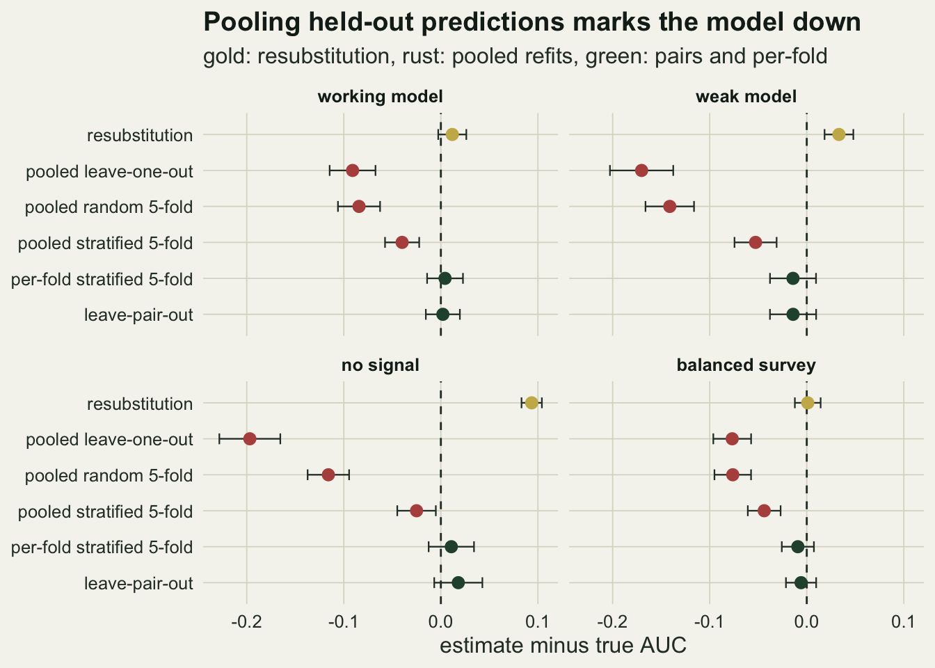
k_weak <- cell_row("weak model", "loo"); k_weak_lpo <- cell_row("weak model", "lpo")
k_null <- cell_row("no signal", "loo"); k_null_lpo <- cell_row("no signal", "lpo")
k_null_pf <- cell_row("no signal", "perfold"); k_null_str <- cell_row("no signal", "strat5")
k_bal <- cell_row("balanced survey", "loo"); k_bal_lpo <- cell_row("balanced survey", "lpo")
weak_below_half <- mean(small_runs[[2]][, "loo"] < 0.5)
weak_truth_below <- mean(small_runs[[2]][, "truth"] < 0.5)
fold_na_share <- mean(small_runs[[1]][, "fold_na"] > 0)
loo_below_lpo <- mean(small_runs[[1]][, "loo"] < small_runs[[1]][, "lpo"])
loo_far_below <- mean(small_runs[[1]][, "loo"] - small_runs[[1]][, "truth"] < -0.1)
The weak model has a conditional AUC of 0.624 and pooled leave-one-out reports 0.454 for it, below one half, while leave-pair-out reports 0.610. In 45 per cent of those surveys the pooled leave-one-out AUC is under one half, although the fitted model is worse than random on new ponds in only 8 per cent of them. A model with some skill is reported as worse than a coin in close to half of the surveys.
With no signal at all, the conditional AUC is 0.499 by construction, and pooled leave-one-out reads 0.303. This is the Parker result: a pooled leave-one-out AUC far below one half is what a null model produces, and reading it as evidence that the covariate works backwards is a mistake. Leave-pair-out reads 0.517, per-fold averaging 0.510, and pooled stratified five-fold 0.474.
The balanced survey is there to test the obvious objection that the bias is a class-imbalance artefact. At an expected occupied share of one half, pooled leave-one-out still reads -0.077 against the truth and leave-pair-out -0.006. Removing any single pond unbalances the other twenty-nine against that pond’s own label whatever the starting share, so balance does not remove it.
Signal makes it a small-sample effect; without signal it fades far more slowly
The next question is whether more ponds cure it. The working model and the null model are rerun at sixty and at one hundred and twenty ponds, with 100 surveys per cell because each survey costs more. The null model gets one more cell, at two hundred and forty ponds, with pooled leave-one-out alone.
n_grid <- c(60, 120); n_ds_big <- 100
set.seed(6021)
t_big <- system.time(
  big_runs <- lapply(c(b_work, b_null), function(bb)
    lapply(n_grid, function(nn) run_cell(n_ds_big, nn, bb, prev_set))))
n_tab <- do.call(rbind, c(
  lapply(1:2, function(j) {
    D30 <- small_runs[[c(1, 3)[j]]]
    cbind(n = n_small, model = c("working model", "no signal")[j], summarise_cell(D30, c("loo", "perfold", "lpo")))
  }),
  lapply(1:2, function(j) do.call(rbind, lapply(1:2, function(m)
    cbind(n = n_grid[m], model = c("working model", "no signal")[j],
          summarise_cell(big_runs[[j]][[m]], c("loo", "perfold", "lpo"))))))))
n_tab$model <- factor(n_tab$model, levels = c("working model", "no signal"))
n_tab$estimator <- factor(est_lab[match(n_tab$estimator, est_code)], levels = est_lab[c(2, 5, 6)])
nb <- function(nn, md) n_tab$bias[n_tab$n == nn & n_tab$model == md & n_tab$estimator == est_lab[2]]
nb_se <- function(nn, md) n_tab$mcse[n_tab$n == nn & n_tab$model == md & n_tab$estimator == est_lab[2]]
# one larger null cell, pooled leave-one-out only: a refit per pond is cheap, 150 pair refits are not
n_null_big <- 240; n_ds_null_big <- 200
loo_only <- function(sv, n_new = 4000) {
  X <- sv$X; y <- sv$y
  cf_all <- fit_logit(X, y)
  Zn <- matrix(rnorm(n_new * sv$p), n_new)
  yn <- rbinom(n_new, 1, plogis(sv$a + sv$b * Zn[, 1]))
  truth <- auc_pairs(cbind(1, Zn) %*% cf_all, yn)
  e <- vapply(seq_along(y), function(i) sum(X[i, ] * fit_logit(X[-i, , drop = FALSE], y[-i])), 0)
  c(truth = truth, loo = auc_pairs(e, y))
}
set.seed(6240)
D240 <- t(replicate(n_ds_null_big, loo_only(draw_survey(n_null_big, b_null, prev_set))))
b240 <- D240[, "loo"] - D240[, "truth"]
n_tab <- rbind(n_tab, data.frame(n = n_null_big, model = "no signal", estimator = est_lab[2],
                                 bias = mean(b240), mcse = sd(b240) / sqrt(n_ds_null_big),
                                 rmse = sqrt(mean(b240^2)), lo = NA, hi = NA, value = mean(D240[, "loo"])))
lpo_big_max <- max(abs(n_tab$bias[n_tab$estimator == est_lab[6]]))
lpo_rows <- rbind(small_tab[small_tab$estimator == est_lab[6], c("bias", "mcse")],
                  n_tab[n_tab$estimator == est_lab[6] & n_tab$n > n_small, c("bias", "mcse")])
lpo_z_max <- max(abs(lpo_rows$bias) / lpo_rows$mcse); n_lpo_cells <- nrow(lpo_rows)
With signal, the pooled leave-one-out bias falls from -0.091 at thirty ponds to -0.046 at sixty and -0.014 at one hundred and twenty (Monte Carlo standard error 0.005 in the last cell). The refit moves each held-out prediction by an amount that shrinks with the number of presences, while the spread of predictions across ponds is set by the slope, which does not shrink, so the tilt becomes small against the gaps it would need to cross.
Without signal the bias is -0.197, -0.172 and -0.172 at thirty, sixty and one hundred and twenty ponds (Monte Carlo standard errors up to 0.022), and -0.119 at two hundred and forty ponds, a cell of 200 surveys where only pooled leave-one-out was run (standard error 0.011). From thirty to one hundred and twenty ponds it does not shrink measurably. By two hundred and forty it has fallen, but it is still 60 per cent of its size at thirty ponds, while with signal the bias at one hundred and twenty ponds is already down to 16 per cent. A null model on a survey eight times larger is still reported well below one half. Part of the reason is that the fitted slope is itself noise here, so the spread of predictions shrinks as the survey grows instead of staying fixed, and the tilt has less to overcome than it does with signal. That heuristic predicts a slow decline rather than none, and the range from thirty to one hundred and twenty ponds alone could not tell the two apart. Leave-pair-out stays within 0.018 of the truth in all six cells where it was run.
The refit, not only the intercept
Parker and colleagues explain the null result through class balance: leaving out a presence lowers the occupied share of the training data, and the intercept follows it. That is one channel. The slope is the other: leaving out an occupied pond at a high covariate value flattens the fitted slope, which lowers the held-out pond’s prediction further. To separate them, the slope-only estimator refits only the slope for each held-out pond and holds the intercept at its value from the full fit, so the class-balance channel is shut.
chan_tab <- do.call(rbind, lapply(seq_len(nrow(small_spec)), function(k) {
  D <- small_runs[[k]]
  data.frame(cell = small_spec$cell[k],
             arm = c("full refit", "slope refitted only"),
             bias = c(mean(D[, "loo"] - D[, "truth"]), mean(D[, "slope_only"] - D[, "truth"])),
             mcse = c(sd(D[, "loo"] - D[, "truth"]), sd(D[, "slope_only"] - D[, "truth"])) / sqrt(nrow(D)))
}))
chan_tab$cell <- factor(chan_tab$cell, levels = small_spec$cell)
chan_share <- vapply(small_spec$cell, function(cl) {
  z <- chan_tab[chan_tab$cell == cl, ]; z$bias[2] / z$bias[1] }, 0)
cb <- function(cl, k) chan_tab$bias[chan_tab$cell == cl][k]
In the working model the full refit gives -0.091 and the slope-only refit -0.024, so with the intercept frozen 27 per cent of the bias remains. In the null model the figures are -0.197 and -0.042, 21 per cent remaining; in the weak model 32 per cent and in the balanced survey 41 per cent. Freezing the intercept removes between 59 and 79 per cent of the bias across the four cells, and what is left, carried by the slope, does not go away. The two channels do not add exactly, since freezing the intercept also changes the slope that is refitted, but the conclusion does not depend on that: the cause is the refit, through every parameter it touches, and a repair that only fixes the class balance of the training data (which is what stratified folds do) leaves part of the bias in place.
p_n <- ggplot(n_tab, aes(n, bias, colour = estimator)) +
  geom_hline(yintercept = 0, colour = te_body, linetype = "dashed", linewidth = 0.5) +
  geom_errorbar(aes(ymin = bias - 2 * mcse, ymax = bias + 2 * mcse), width = 6, linewidth = 0.4) +
  geom_line(linewidth = 0.9) + geom_point(size = 2.2) +
  facet_wrap(~model, ncol = 2, scales = "free_x") +
  scale_x_continuous(breaks = c(n_small, n_grid, n_null_big)) +
  scale_colour_manual(values = c(te_rust, te_sage, te_forest), name = NULL) +
  guides(colour = guide_legend(nrow = 2)) +
  labs(x = "ponds in the survey", y = "estimate minus true AUC", title = "More ponds",
       subtitle = "the bias fades fast with signal, slowly without") +
  theme_datasheet() + theme(legend.position = "bottom",
                            strip.text = element_text(colour = te_ink, face = "bold"))
p_chan <- ggplot(chan_tab, aes(bias, cell, fill = arm)) +
  geom_vline(xintercept = 0, colour = te_body, linetype = "dashed", linewidth = 0.5) +
  geom_col(position = position_dodge(width = 0.7), width = 0.6, colour = te_paper, linewidth = 0.3) +
  scale_fill_manual(values = c(te_rust, te_gold), name = NULL) +
  scale_y_discrete(limits = rev(levels(chan_tab$cell))) +
  guides(fill = guide_legend(nrow = 2)) +
  labs(x = "estimate minus true AUC", y = NULL, title = "Two channels",
       subtitle = "thirty ponds, pooled leave-one-out") +
  theme_datasheet() + theme(legend.position = "bottom")
p_n + p_chan + plot_layout(widths = c(1.6, 1)) + plot_annotation(theme = theme_datasheet())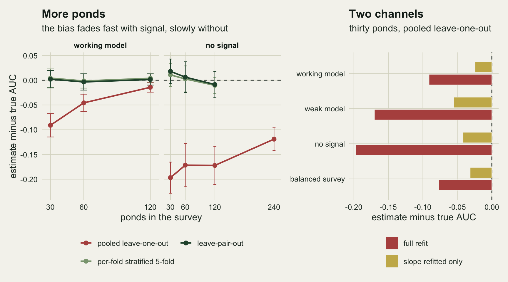
With extra covariates, resubstitution stops being honest
A single covariate made resubstitution look unbiased, which would teach the wrong lesson: that leave-one-out is worse than not validating at all. Real models carry more than one covariate, and most of the candidates on a pond survey (area, shade, fish, distance to a road) do less than the analyst hopes. So the model is refitted with the working habitat covariate plus four more that have no effect at all in the generating process, all five entered into the logistic regression, at thirty and at sixty ponds. Six coefficients on about nine presences can separate, which sends a maximum-likelihood fit off towards infinite coefficients (see Bayesian logistic regression under separation and the section “Where a small presence count really does bite” of class imbalance in species presence models), so the share of fits with fitted probabilities at 0 or 1 to machine precision is recorded for the full fit and for every leave-one-out refit. The rule, fixed before the run: if more than a fifth of the full fits at thirty ponds separate, the arm moves to two noise covariates.
n_noise <- 4; sep_limit <- 0.2
set.seed(7755)
t_multi <- system.time(
  multi_runs <- list(run_cell(n_ds_small, n_small, b_work, prev_set, n_noise),
                     run_cell(n_ds_big, 60, b_work, prev_set, n_noise)))
multi_n <- c(n_small, 60)
multi_tab <- do.call(rbind, lapply(1:2, function(m)
  cbind(ponds = sprintf("%d ponds", multi_n[m]), summarise_cell(multi_runs[[m]]))))
multi_tab$ponds <- factor(multi_tab$ponds, levels = sprintf("%d ponds", multi_n))
multi_tab$estimator <- factor(est_lab[match(multi_tab$estimator, est_code)], levels = rev(est_lab))
mr <- function(m, est) multi_tab[multi_tab$ponds == sprintf("%d ponds", multi_n[m]) &
                                 multi_tab$estimator == est_lab[match(est, est_code)], ]
sep_full30 <- mean(multi_runs[[1]][, "edge_full"]); sep_loo30 <- mean(multi_runs[[1]][, "edge_loo"])
sep_full60 <- mean(multi_runs[[2]][, "edge_full"])
truth_multi <- vapply(multi_runs, function(D) mean(D[, "truth"]), 0)
m_sep <- multi_runs[[1]][, "edge_full"] == 1
lpo_bias_nosep <- mean(multi_runs[[1]][!m_sep, "lpo"] - multi_runs[[1]][!m_sep, "truth"])
res_bias_nosep <- mean(multi_runs[[1]][!m_sep, "resub"] - multi_runs[[1]][!m_sep, "truth"])
D30 <- multi_runs[[1]]
sq_diff <- (D30[, "perfold"] - D30[, "truth"])^2 - (D30[, "lpo"] - D30[, "truth"])^2
sq_diff_mean <- mean(sq_diff, na.rm = TRUE); sq_diff_se <- sd(sq_diff, na.rm = TRUE) / sqrt(sum(!is.na(sq_diff)))
# squared error of a pooled estimator minus that of per-fold averaging, per survey
sq_vs_pf <- function(est) {
  d <- (D30[, est] - D30[, "truth"])^2 - (D30[, "perfold"] - D30[, "truth"])^2
  c(mean = mean(d, na.rm = TRUE), se = sd(d, na.rm = TRUE) / sqrt(sum(!is.na(d))))
}
sq_str <- sq_vs_pf("strat5"); sq_loo <- sq_vs_pf("loo")
At thirty ponds 4.0 per cent of the full fits and 4.8 per cent of the leave-one-out refits separate, under the fifth set as the limit, so the arm keeps its four noise covariates; at sixty ponds the full-fit share is 0.0 per cent. The noise covariates cost the model real skill: its conditional AUC averages 0.673 at thirty ponds and 0.716 at sixty, against 0.751 for the one-covariate model at thirty.
Resubstitution is now optimistic, at +0.170 at thirty ponds and +0.085 at sixty. Pooled leave-one-out is pessimistic, at -0.077 and -0.035. Leave-pair-out sits between them at -0.005 and +0.003, and per-fold averaging at -0.015 and +0.001. Dropping the separated surveys changes little: leave-pair-out then reads -0.013 and resubstitution +0.164 at thirty ponds.
Bias is not the only property that matters for one survey, since an unbiased estimator with a wide spread still misleads on the survey in hand. Folds with one or two presences give noisy AUCs, and averaging five of them might be expected to be noisier than scoring 150 pairs. At thirty ponds the root mean squared error against the truth is 0.134 for leave-pair-out, 0.146 for per-fold averaging, 0.148 for pooled stratified five-fold, 0.162 for pooled leave-one-out, 0.170 for pooled random five-fold and 0.192 for resubstitution. Leave-pair-out has the smallest error of the six. Per survey, the squared error of per-fold averaging exceeds that of leave-pair-out by 0.0032 on average, with a standard error of 0.0014, so per-fold averaging is a little noisier at nine presences and five covariates, as the folds with one or two presences suggest it should be. Its error is not measurably smaller than that of pooled stratified five-fold, whose squared error is larger by only 0.0006 (standard error 0.0013): that estimator’s trouble is bias rather than spread. Pooled leave-one-out’s squared error exceeds that of per-fold averaging by 0.0052 (standard error 0.0020), and resubstitution has the largest error of all.
ggplot(multi_tab, aes(bias, estimator)) +
  geom_vline(xintercept = 0, colour = te_body, linetype = "dashed", linewidth = 0.5) +
  geom_errorbar(aes(xmin = bias - 2 * mcse, xmax = bias + 2 * mcse), orientation = "y",
                width = 0.3, colour = te_body, linewidth = 0.4) +
  geom_point(aes(colour = estimator), size = 2.6) +
  scale_colour_manual(values = est_col, guide = "none") +
  facet_wrap(~ponds, ncol = 2) +
  labs(x = "estimate minus true AUC", y = NULL,
       title = "Resubstitution flatters, pooling marks down",
       subtitle = "gold: resubstitution, rust: pooled refits, green: pairs and per-fold") +
  theme_datasheet() + theme(strip.text = element_text(colour = te_ink, face = "bold"))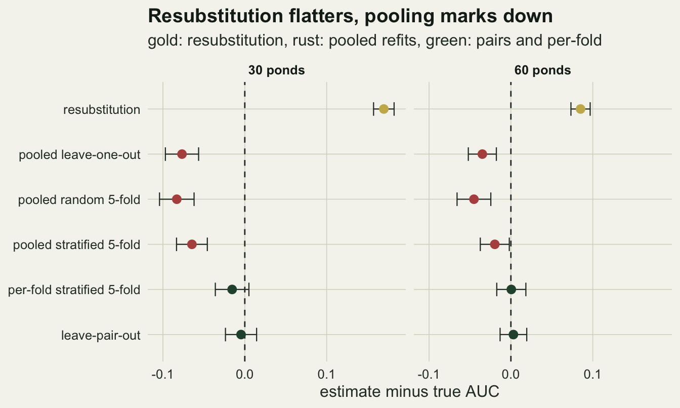
Why the spatial post can pool, and when a large survey cannot
The size of the tilt is set by how much information the fit has, and for a rare species that is close to the number of presences, not the number of sites. The intercept’s score equation says that the fitted probabilities must sum to the number of presences; remove one presence and they must sum to one less, so through the intercept alone the pond’s own linear predictor moves by about one minus its fitted probability divided by the sum of the binomial weights, which is close to one over that sum for a rare species. The slope adds to that, and adds more the further the pond’s covariate value lies from the weighted centre of the data. Both scale with the information in the fit, and for a rare species the sum of weights is close to the number of presences. Three settings test that directly: thirty ponds at an occupied share of three in ten, 1500 sites at the same share (the scale of the spatial cross-validation post, with the working slope; its GAM is not refitted here), and 1000 sites at an occupied share of one in a hundred, which gives about ten presences among a large number of absences, the shape of a presence-background data set.
tilt_setting <- function(n, prev, reps, n_abs = 30) {
  out <- replicate(reps, {
    sv <- draw_survey(n, b_work, prev)
    X <- sv$X; y <- sv$y; cf <- fit_logit(X, y); eta <- drop(X %*% cf)
    P <- which(y == 1); A <- which(y == 0)
    A <- A[sample.int(length(A), min(n_abs, length(A)))]
    own <- function(i) eta[i] - sum(X[i, ] * fit_logit(X[-i, , drop = FALSE], y[-i]))
    w <- plogis(eta) * (1 - plogis(eta))
    c(n1 = sum(y), pres = mean(vapply(P, own, 0)), abs = -mean(vapply(A, own, 0)),
      spread = sd(eta), info = sum(w))
  })
  rowMeans(out)
}
set.seed(9150)
tilt_tab <- rbind(small = tilt_setting(n_small, prev_set, 20),
                  large = tilt_setting(1500, prev_set, 2),
                  rare  = tilt_setting(1000, 0.01, 10))
n_cv <- 1500; n_ds_cv <- 40
set.seed(9151)
cv_big <- t(replicate(n_ds_cv, {
  sv <- draw_survey(n_cv, b_work, prev_set); X <- sv$X; y <- sv$y
  cf <- fit_logit(X, y)
  Zn <- matrix(rnorm(4000), 4000); yn <- rbinom(4000, 1, plogis(sv$a + sv$b * Zn[, 1]))
  folds <- sample(rep(1:5, length.out = n_cv)); s <- numeric(n_cv)
  for (k in 1:5) { te <- folds == k; s[te] <- X[te, ] %*% fit_logit(X[!te, ], y[!te]) }
  c(auc_pairs(s, y), auc_pairs(cbind(1, Zn) %*% cf, yn))
}))
cv_big_bias <- mean(cv_big[, 1] - cv_big[, 2])
cv_big_se <- sd(cv_big[, 1] - cv_big[, 2]) / sqrt(n_ds_cv)
On thirty ponds with 10.0 presences on average, leaving a presence out lowers its own linear predictor by 0.243 and leaving an absence out raises its own by 0.117, against a spread of 1.31 across ponds and a sum of weights of 5.0, whose inverse is 0.198. On 1500 sites with 450 presences the same shifts are 0.0044 and 0.0016, with a sum of weights of 265: one row barely moves the refit. Pooled random five-fold on 40 such surveys has a bias of -0.0031 (Monte Carlo standard error 0.0024), so the spatial post was right to pool.
The rare-species survey is the case to worry about. With 1000 sites but only 10.9 presences on average, leaving a presence out lowers its own predictor by 0.253, as much as on thirty ponds. The sum of weights is 10.5, close to the number of presences, and the shift is 2.6 times its inverse of 0.096: the intercept accounts for part of it and the slope for the rest. The absences hardly move (0.0020), so the tilt now falls almost entirely on the presences. A large survey does not protect a rare species; many presences do.
What to report
Report how the AUC was computed, not only that it was cross-validated. Pooled leave-one-out, pooled k-fold, per-fold averaging and leave-pair-out are four different estimators, and on a survey with nine presences they disagree by close to a tenth on the AUC scale in the working model measured here. The gap is not an average hiding a spread of signs either: pooled leave-one-out came in below leave-pair-out in 99 per cent of those surveys, and more than 0.1 below the truth in 39 per cent. Forman and Scholz 2010 make the same point for machine-learning benchmarks, where pooling and averaging across folds is a common silent difference between papers that claim to use the same protocol.
On a small presence-absence survey, score pairs or average per fold, and never pool leave-one-out predictions into one AUC. Leave-pair-out is the safer of the two when presences are few. In the five-covariate arm its squared error per survey was smaller by 0.0032 (standard error 0.0014), and a stratified fold needs at least one presence to have an AUC at all; 1.5 per cent of the working-model surveys at thirty ponds had a fold without one.
Give the number of presences next to any cross-validated AUC. It sets the size of the tilt, and a reader who sees nine presences knows to ask which estimator was used; a reader who sees 1000 sites does not, even though a rare species in a large survey carries the same tilt.
Report resubstitution beside the cross-validated figure when the model has more than one covariate, and read the gap. The honest number lies below resubstitution and above pooled leave-one-out; if the two bracket a value near one half, the model may have no skill, and a pooled leave-one-out figure well below one half is itself a sign of that, not of a covariate working backwards.
Honest limits
Everything here is a logistic regression with normally distributed covariates and a correctly specified working term. A flexible model (a GAM, a boosted tree, MaxEnt) refits many more parameters, and often chooses how many, and each extra degree of freedom is another channel through which the held-out label can tilt the refit, so the bias of pooled leave-one-out is unlikely to be smaller there; but that was not measured, and neither was how far leave-pair-out stays unbiased for a model that selects its own complexity inside each refit.
The truth is the conditional AUC of the model fitted to all ponds. Cross-validation estimates the performance of models fitted to fewer rows, which are slightly worse, so an estimator can be pessimistic against this truth for a fair reason. The size of that fair gap here is bounded by what leave-pair-out shows, since it refits on two ponds fewer than the full model and stays within 1.5 Monte Carlo standard errors of the truth in the 8 one-covariate cells; the pooled estimators are pessimistic by far more.
Pearson and colleagues 2007 validated species models built from four to twenty-three locality records with a jackknife that scores each held-out presence against a threshold, not with an AUC. The tilt measured here lowers each held-out presence’s own prediction, which should lower the share of presences that clear a fixed threshold as well, but the threshold version was not simulated and the size of that effect is unknown.
For presence-background models the one-row section shows that the tilt on a held-out presence does not shrink with the size of the background. What was not measured is the AUC consequence under the usual presence-background protocol, where only presences are held out and the background is scored by a single model; there the tilt falls on one class only, and the bias is likely to be at least as large, but that is an expectation, not a result.
The replication is 200 surveys per cell at thirty ponds and 100 at sixty and one hundred and twenty (200 in the null cell at two hundred and forty, pooled leave-one-out only), with a leave-pair-out sample of 150 pairs per survey. The Monte Carlo standard errors are printed with every bias; differences between the unbiased estimators smaller than about two of them are not worth interpreting.
References
Parker BJ, Gunter S, Bedo J 2007 BMC Bioinformatics 8:326 (10.1186/1471-2105-8-326)
Airola A, Pahikkala T, Waegeman W, De Baets B, Salakoski T 2011 Computational Statistics and Data Analysis 55(4):1828-1844 (10.1016/j.csda.2010.11.018)
Forman G, Scholz M 2010 ACM SIGKDD Explorations Newsletter 12(1):49-57 (10.1145/1882471.1882479)
Pearson RG, Raxworthy CJ, Nakamura M, Peterson AT 2007 Journal of Biogeography 34(1):102-117 (10.1111/j.1365-2699.2006.01594.x)