Smoothing a series before testing a forecast

Smoothing a population index over the whole record flatters a one-step hindcast in R. Refitted at each forecast origin, the same smoother loses to raw AR(1).

A farmland bird index runs for forty years. The annual values jump about, partly because the population really does move and partly because a count is a count: a wet May, a new observer, a route that was not walked. The usual first step is to smooth it, with a GAM through the years or a spline with degrees of freedom set to three tenths of the series length, the rule Fewster and colleagues used for farmland bird trends in 2000. The smooth looks like the population, so it is natural to forecast from it: fit a first-order autoregression to the smoothed index, predict next year, and check the method by hindcasting the last fifteen years one step at a time. The hindcast says smoothing helps.

That hindcast has a leak in it, and the repair is not new. Tashman’s 2000 review of out-of-sample forecast tests describes rolling-origin evaluation: each forecast is made from an origin, with only the data available at that origin. The site’s own post on data leakage in model validation states the general rule in its section on preprocessing: “Anything that consults the response is a different case … Those belong inside the fold; the rest belong there for tidiness.” A smoother fitted to the whole record consults the response, because in a series the response is the next value of the same series. Inside the fold, in time order, means using only the years before the forecast origin. So the repair is to refit the smoother at every origin on the years available then, and forecast from its endpoint.

What this post measures is the price of that repair. The data-leakage post shows a leak that inflates a score and a leak-free version that deflates it back to the truth. Here the leak-free version does not just shrink the gain from smoothing, it reverses it: the smoother done honestly, in the same pipeline, forecasts worse than no smoother at all. The verdict flips. That is related to, but not the same as, the flip in forecast skill and the baseline, where one forecast is judged skilful or useless depending on the reference; here the reference is fixed and the construction of the predictor is what changes. The same future-in-the-predictor problem turns up inside a delay embedding in simplex projection and delay embedding, where the theiler exclusion is the repair; a smoothed index is the version a population ecologist is more likely to meet.

A population index with counting error

The generating model is the Gompertz log index from the Gompertz state-space model: the true log abundance follows a first-order autoregression with coefficient 0.7 and process standard deviation 0.15, and each year’s observed index adds independent counting error. Each series is forty years long, starting from the stationary distribution. The first twenty five years are the training period; the hindcast makes fifteen one-step forecasts, from origins at years 25 to 39, each for the following year. Every arm is refitted at every origin, on an expanding window.

library(ggplot2)
library(patchwork)
library(mgcv)

te_paper  <- "#f5f4ee"
te_ink    <- "#16241d"
te_body   <- "#2c3a31"
te_forest <- "#275139"
te_rust   <- "#b5534e"
te_gold   <- "#c9b458"
te_line   <- "#dad9ca"

theme_datasheet <- function() {
  theme_minimal(base_size = 12) +
    theme(plot.background  = element_rect(fill = te_paper, colour = NA),
          panel.background = element_rect(fill = te_paper, colour = NA),
          panel.grid.major = element_line(colour = te_line, linewidth = 0.3),
          panel.grid.minor = element_blank(),
          text             = element_text(colour = te_body),
          plot.title       = element_text(colour = te_ink, face = "bold"),
          plot.subtitle    = element_text(colour = te_body),
          axis.text        = element_text(colour = te_body))
}

n_year  <- 40       # years in each series
n_train <- 25       # training years before the first origin
b_true  <- 0.7      # density dependence on the log scale
sd_proc <- 0.15     # process standard deviation
sd_obs_main <- 0.25 # counting error, main cell
origins <- n_train:(n_year - 1)

sim_index <- function(sd_obs, n = n_year) {
  x <- numeric(n)
  x[1] <- rnorm(1, 0, sd_proc / sqrt(1 - b_true^2))
  for (i in 2:n) x[i] <- b_true * x[i - 1] + rnorm(1, 0, sd_proc)
  eps <- rnorm(n, 0, sd_obs)
  list(x = x, y = x + eps, eps = eps)
}

# least squares AR(1) fitted on s[1:t]: forecast of year t + 1 from s[t], and the slope
ar_fit <- function(s, t) {
  z0 <- s[1:(t - 1)]; z1 <- s[2:t]
  ok <- is.finite(z0) & is.finite(z1); z0 <- z0[ok]; z1 <- z1[ok]
  slope <- sum((z0 - mean(z0)) * (z1 - mean(z1))) / sum((z0 - mean(z0))^2)
  c(mean(z1) + slope * (s[t] - mean(z0)), slope)
}
ar_step <- function(s, t) ar_fit(s, t)[1]
spline_fit <- function(y, dof) predict(smooth.spline(seq_along(y), y, df = dof), seq_along(y))$y
mean3_centred  <- function(y) { n <- length(y); c(NA, (y[1:(n - 2)] + y[2:(n - 1)] + y[3:n]) / 3, NA) }
mean3_trailing <- function(y) { n <- length(y); c(NA, NA, (y[1:(n - 2)] + y[2:(n - 1)] + y[3:n]) / 3) }
reml_fit <- function(y) {
  dd <- data.frame(yr = seq_along(y), y = y)
  fitted(gam(y ~ s(yr, k = min(20, length(y) - 2)), data = dd, method = "REML"))
}

The smoothers are the ones in use for population indices: smooth.spline at 4, 8 and 12 degrees of freedom (12 is three tenths of 40, the Fewster rule), a three-year running mean, and a thin plate s(year) in mgcv with its smoothness chosen by REML. Each appears twice. The leaky arm smooths all forty years once and then, at each origin, fits the autoregression to the smoothed values up to the origin and forecasts from the smoothed value at the origin. The real-time arm smooths only the years up to the origin and forecasts from the endpoint of that smooth; for the running mean the real-time version is the trailing mean of the last three years. The reference is the same autoregression fitted to the raw index.

one_series <- function(sd_obs, dofs, do_reml = FALSE) {
  d <- sim_index(sd_obs); y <- d$y; x <- d$x
  fc <- list(); base <- list(); slp <- list()  # forecast, value it starts from, AR slope
  add_leaky <- function(nm, s) {
    m <- sapply(origins, function(t) ar_fit(s, t))
    fc[[nm]] <<- m[1, ]; slp[[nm]] <<- m[2, ]; base[[nm]] <<- s[origins]
  }
  add_realtime <- function(nm, fitter) {
    m <- sapply(origins, function(t) { s <- fitter(y[1:t]); c(ar_fit(s, t), s[t]) })
    fc[[nm]] <<- m[1, ]; slp[[nm]] <<- m[2, ]; base[[nm]] <<- m[3, ]
  }
  for (dof in dofs) {
    add_leaky(paste0("leaky spline df ", dof), spline_fit(y, dof))
    add_realtime(paste0("real-time spline df ", dof), function(z) spline_fit(z, dof))
  }
  add_leaky("leaky 3-year mean", mean3_centred(y))
  add_leaky("real-time 3-year mean", mean3_trailing(y))  # one-sided already
  if (do_reml) {
    add_leaky("leaky REML GAM", reml_fit(y))
    add_realtime("real-time REML GAM", reml_fit)
  }
  add_leaky("raw", y)
  fc$persistence <- y[origins]; base$persistence <- y[origins]; slp$persistence <- rep(1, length(origins))
  fc$oracle <- b_true * x[origins]; base$oracle <- x[origins]; slp$oracle <- rep(b_true, length(origins))
  ty <- y[origins + 1]; tx <- x[origins + 1]; te <- d$eps[origins + 1]
  sapply(names(fc), function(nm) {
    p <- fc[[nm]]; bs <- base[[nm]]
    c(sy = sum((p - ty)^2), sx = sum((p - tx)^2), cr = sum((p - tx) * te),
      sb = sum((bs - x[origins])^2), sl = sum(slp[[nm]]),
      b1 = sum(bs), b2 = sum(bs^2), by = sum(bs * ty), y1 = sum(ty), n = length(p))
  })
}
run_batch <- function(n_ser, ...) Reduce(`+`, lapply(seq_len(n_ser), function(i) one_series(...)))

cell_long <- function(L) do.call(rbind, lapply(seq_along(L), function(k) {
  m <- L[[k]]
  data.frame(arm = colnames(m), batch = k,
             rmse_y = sqrt(m["sy", ] / m["n", ]), rmse_x = sqrt(m["sx", ] / m["n", ]),
             base_err = sqrt(m["sb", ] / m["n", ]),
             ratio_raw = sqrt(m["sy", ] / m["sy", "raw"]),
             ratio_oracle = sqrt(m["sy", ] / m["sy", "oracle"]))
}))
q3 <- function(tab, a, col) { v <- tab[tab$arm == a, col]; c(median(v), min(v), max(v)) }
f3 <- function(v, dg = 3) sprintf("%.*f [%.*f, %.*f]", dg, v[1], dg, v[2], dg, v[3])
pct <- function(r) 100 * abs(1 - r)

Every score below is a root mean squared error over the fifteen test years of every series in a batch, scored against the observed index of the following year, because the observed index is what a reader has to score against. The headline number is the ratio of an arm’s error to the raw autoregression’s error on the same series; below one means the arm looks better. The design constants and the replication (five batches per cell, reported as the median batch with the range over batches in brackets) were fixed before any arm was run.

What the whole-record smooth knows at the origin

A spline with its degrees of freedom fixed is a linear smoother: each smoothed value is a weighted sum of all forty observed values, and the weights depend only on the years, not on the counts. That makes the leak something that can be read off directly, by smoothing a vector with a one in a single year and zeros elsewhere.

smooth_row <- function(fitter, t, n = n_year) {
  vapply(seq_len(n), function(j) { e <- numeric(n); e[j] <- 1; fitter(e)[t] }, 0)
}
t_show <- 30
w_list <- lapply(c(4, 8, 12), function(dof) smooth_row(function(z) spline_fit(z, dof), t_show))
set.seed(3001)
y_chk <- rnorm(n_year)
lin_gap <- max(vapply(seq_along(w_list), function(i)
  abs(sum(w_list[[i]] * y_chk) - spline_fit(y_chk, c(4, 8, 12)[i])[t_show]), 0))
w_next <- vapply(w_list, function(w) w[t_show + 1], 0)
w_future <- vapply(w_list, function(w) sum(w[(t_show + 1):n_year]), 0)
w_own <- vapply(w_list, function(w) w[t_show], 0)

At year 30, which is the origin for forecasting year 31, the whole-record spline gives year 31 a weight of 0.077 at 4 degrees of freedom, 0.159 at 8 and 0.219 at 12, and all the years after the origin together carry 0.44, 0.41 and 0.36 of the total. The centred three-year mean gives the next year one third, by construction. The weights reproduce the fitted spline on an arbitrary series to within floating-point rounding, so they are the smoother and not an approximation of it. The REML GAM has no such fixed weights, because its smoothness is chosen from the data, but it is a two-sided smoother of the same kind.

So the value the autoregression forecasts from already contains a fraction of the very number it is being scored against. That fraction carries two things: part of next year’s real change in the population, and the same share of next year’s counting error. The second is pure leak; no forecaster can know it in advance.

set.seed(3030)
ex <- sim_index(sd_obs_main)
ex_all <- spline_fit(ex$y, 12)
ex_rt  <- spline_fit(ex$y[1:t_show], 12)
ex_fc_leak <- ar_step(ex_all, t_show)
ex_fc_rt   <- ar_step(ex_rt, t_show)
ex_fc_raw  <- ar_step(ex$y, t_show)
ex_target  <- ex$y[t_show + 1]

ex_df <- data.frame(year = seq_len(n_year), y = ex$y, x = ex$x, s_all = ex_all,
                    s_rt = c(ex_rt, rep(NA, n_year - t_show)))
fc_df <- data.frame(year = t_show + 1,
                    val = c(ex_fc_leak, ex_fc_rt, ex_fc_raw),
                    arm = factor(c("from the whole-record smooth", "from the real-time smooth",
                                   "from the raw index"),
                                 levels = c("from the whole-record smooth",
                                            "from the real-time smooth", "from the raw index")))
ggplot(ex_df, aes(year)) +
  annotate("rect", xmin = t_show + 0.5, xmax = n_year + 0.5, ymin = -Inf, ymax = Inf,
           fill = te_line, alpha = 0.45) +
  geom_line(aes(y = x), colour = te_gold, linewidth = 0.6, linetype = "dashed") +
  geom_point(aes(y = y), colour = te_ink, size = 1.6) +
  geom_line(aes(y = s_all), colour = te_rust, linewidth = 0.9) +
  geom_line(aes(y = s_rt), colour = te_forest, linewidth = 0.9, na.rm = TRUE) +
  geom_point(data = data.frame(year = t_show + 1, y = ex_target), aes(y = y),
             shape = 21, size = 5, stroke = 1, colour = te_ink, fill = NA) +
  geom_point(data = fc_df, aes(year + c(0.35, 0.35, 0.35), val, shape = arm, colour = arm),
             size = 2.8, stroke = 1) +
  scale_shape_manual(values = c(17, 15, 4), name = NULL) +
  scale_colour_manual(values = c(te_rust, te_forest, te_ink), name = NULL) +
  guides(shape = guide_legend(nrow = 3), colour = guide_legend(nrow = 3)) +
  labs(x = "year", y = "log index",
       title = "The whole-record smooth has seen year 31",
       subtitle = "rust: spline on all 40 years; green: spline on years 1 to 30; dashed gold: true state") +
  theme_datasheet() + theme(legend.position = "bottom")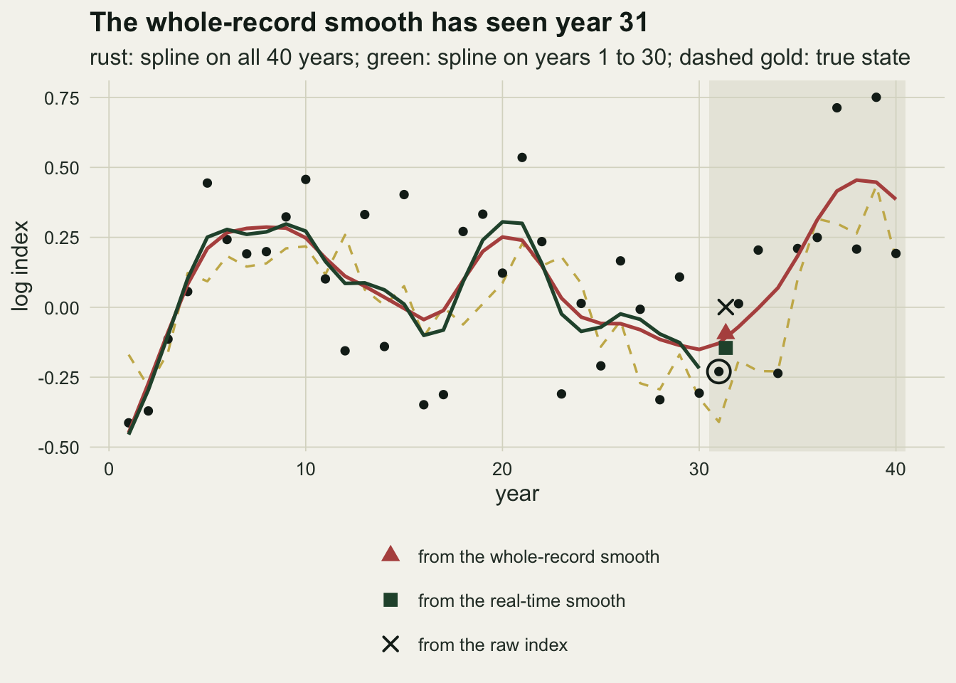

Figure 1: One simulated index with the 12 degree of freedom spline fitted to all forty years and the same spline fitted only to the years up to the origin at year 30, with the one-step forecasts each produces for year 31.

In this series the observed index for year 31 is -0.230. The forecast from the whole-record smooth is -0.095, from the real-time smooth -0.145 and from the raw index 0.001. Here the real-time forecast happens to land closer to the target than the leaky one, which is one year of one series and proves nothing on its own; the next section repeats this for every origin of many series.

The leaky hindcast and the honest one disagree

n_batch <- 5; n_per_batch <- 100      # fixed before any arm was run
set.seed(2510)
L_main <- lapply(seq_len(n_batch), function(k) run_batch(n_per_batch, sd_obs_main, c(4, 8, 12)))
tab_main <- cell_long(L_main)
arm_pairs <- data.frame(
  smoother = c("spline df 4", "spline df 8", "spline df 12", "3-year mean"),
  leaky = c("leaky spline df 4", "leaky spline df 8", "leaky spline df 12", "leaky 3-year mean"),
  realtime = c("real-time spline df 4", "real-time spline df 8", "real-time spline df 12",
               "real-time 3-year mean"))
r_leak <- sapply(arm_pairs$leaky, function(a) q3(tab_main, a, "ratio_raw"))
r_rt   <- sapply(arm_pairs$realtime, function(a) q3(tab_main, a, "ratio_raw"))
raw_main <- q3(tab_main, "raw", "rmse_y"); orc_main <- q3(tab_main, "oracle", "rmse_y")
per_main <- q3(tab_main, "persistence", "ratio_raw")
n_series_main <- n_batch * n_per_batch
leak_hi <- max(r_leak[3, 1:3])   # worst batch of any leaky spline
rt_lo   <- min(r_rt[2, 1:3])     # best batch of any real-time spline

Across 500 series with counting error of standard deviation 0.25, the raw autoregression scores 0.325 [0.314, 0.328]. Against that, the leaky arms give ratios of 0.863 [0.851, 0.875] for the spline at 4 degrees of freedom, 0.793 [0.782, 0.804] at 8, 0.772 [0.759, 0.783] at 12 and 0.750 [0.735, 0.756] for the centred three-year mean. Read as a hindcast, smoothing cuts forecast error by 14 to 25 per cent, and the more the smoother leans on the next year, the better it looks: the ordering follows the weight each smoother puts on the next year, from the previous section.

The real-time arms, the same smoothers refitted at each origin on the years available then, give 1.071 [1.045, 1.078], 1.106 [1.086, 1.121], 1.106 [1.087, 1.125] and 1.016 [1.002, 1.026]. Every spline is worse than no smoothing, by 7 to 11 per cent, and the trailing mean is 1.6 per cent worse. No batch of any spline arm lands on the other side of one, in either direction: the worst leaky spline batch is 0.875 and the best real-time spline batch 1.045. For scale, forecasting next year as this year’s value, the persistence baseline, gives a ratio of 1.201 [1.172, 1.246].

n_per_batch_reml <- 20                # fixed before any arm was run
set.seed(2520)
L_reml <- lapply(seq_len(n_batch), function(k)
  run_batch(n_per_batch_reml, sd_obs_main, numeric(0), do_reml = TRUE))
tab_reml <- cell_long(L_reml)
r_reml_leak <- q3(tab_reml, "leaky REML GAM", "ratio_raw")
r_reml_rt   <- q3(tab_reml, "real-time REML GAM", "ratio_raw")
o_reml_leak <- q3(tab_reml, "leaky REML GAM", "ratio_oracle")
n_reml_above <- sum(tab_reml$ratio_oracle[tab_reml$arm == "leaky REML GAM"] > 1)
o_leak_main <- sapply(arm_pairs$leaky, function(a) q3(tab_main, a, "ratio_oracle"))
n_series_reml <- n_batch * n_per_batch_reml

The GAM has to be fitted sixteen times per series and is slow, so it gets its own cell of 100 series. Smoothed over the whole record it looks 17 per cent better than raw, ratio 0.826 [0.818, 0.878]. Refitted at each origin it is 8 per cent worse, ratio 1.080 [1.057, 1.107]. Choosing the smoothness from the data does not rescue the real-time smoother.

ver <- do.call(rbind, lapply(seq_len(nrow(arm_pairs)), function(i) rbind(
  data.frame(smoother = arm_pairs$smoother[i], use = "whole record (leaky)",
             ref = "relative to raw AR(1)", t(q3(tab_main, arm_pairs$leaky[i], "ratio_raw"))),
  data.frame(smoother = arm_pairs$smoother[i], use = "real time (honest)",
             ref = "relative to raw AR(1)", t(q3(tab_main, arm_pairs$realtime[i], "ratio_raw"))),
  data.frame(smoother = arm_pairs$smoother[i], use = "whole record (leaky)",
             ref = "relative to the oracle", t(q3(tab_main, arm_pairs$leaky[i], "ratio_oracle"))),
  data.frame(smoother = arm_pairs$smoother[i], use = "real time (honest)",
             ref = "relative to the oracle", t(q3(tab_main, arm_pairs$realtime[i], "ratio_oracle"))))))
ver <- rbind(ver,
  data.frame(smoother = "REML GAM", use = "whole record (leaky)", ref = "relative to raw AR(1)",
             t(r_reml_leak)),
  data.frame(smoother = "REML GAM", use = "real time (honest)", ref = "relative to raw AR(1)",
             t(r_reml_rt)),
  data.frame(smoother = "REML GAM", use = "whole record (leaky)", ref = "relative to the oracle",
             t(o_reml_leak)),
  data.frame(smoother = "REML GAM", use = "real time (honest)", ref = "relative to the oracle",
             t(q3(tab_reml, "real-time REML GAM", "ratio_oracle"))))
names(ver)[4:6] <- c("med", "lo", "hi")
ver$smoother <- factor(ver$smoother, levels = rev(c(arm_pairs$smoother, "REML GAM")))
ver$use <- factor(ver$use, levels = c("whole record (leaky)", "real time (honest)"))
ref_lines <- data.frame(ref = c("relative to raw AR(1)", "relative to the oracle"), at = 1)
plot_verdict <- function(dat) {
  ggplot(dat, aes(med, smoother, colour = use, shape = use)) +
    geom_vline(data = ref_lines[ref_lines$ref %in% dat$ref, ], aes(xintercept = at),
               colour = te_body, linetype = "dashed", linewidth = 0.5) +
    geom_errorbar(aes(xmin = lo, xmax = hi), orientation = "y", width = 0.25,
                  linewidth = 0.5, position = position_dodge(width = 0.5)) +
    geom_point(size = 2.6, position = position_dodge(width = 0.5)) +
    scale_colour_manual(values = c(te_rust, te_forest), name = NULL) +
    scale_shape_manual(values = c(17, 16), name = NULL) +
    labs(x = "RMSE ratio", y = NULL) +
    theme_datasheet() + theme(legend.position = "bottom")
}
p_raw <- plot_verdict(ver[ver$ref == "relative to raw AR(1)", ]) +
  labs(title = "Against no smoothing", subtitle = "dashed line: raw AR(1)")
p_orc <- plot_verdict(ver[ver$ref == "relative to the oracle", ]) +
  labs(title = "Against the oracle", subtitle = "dashed line: the oracle")
p_raw + p_orc + plot_layout(guides = "collect") +
  plot_annotation(theme = theme_datasheet() + theme(legend.position = "bottom"))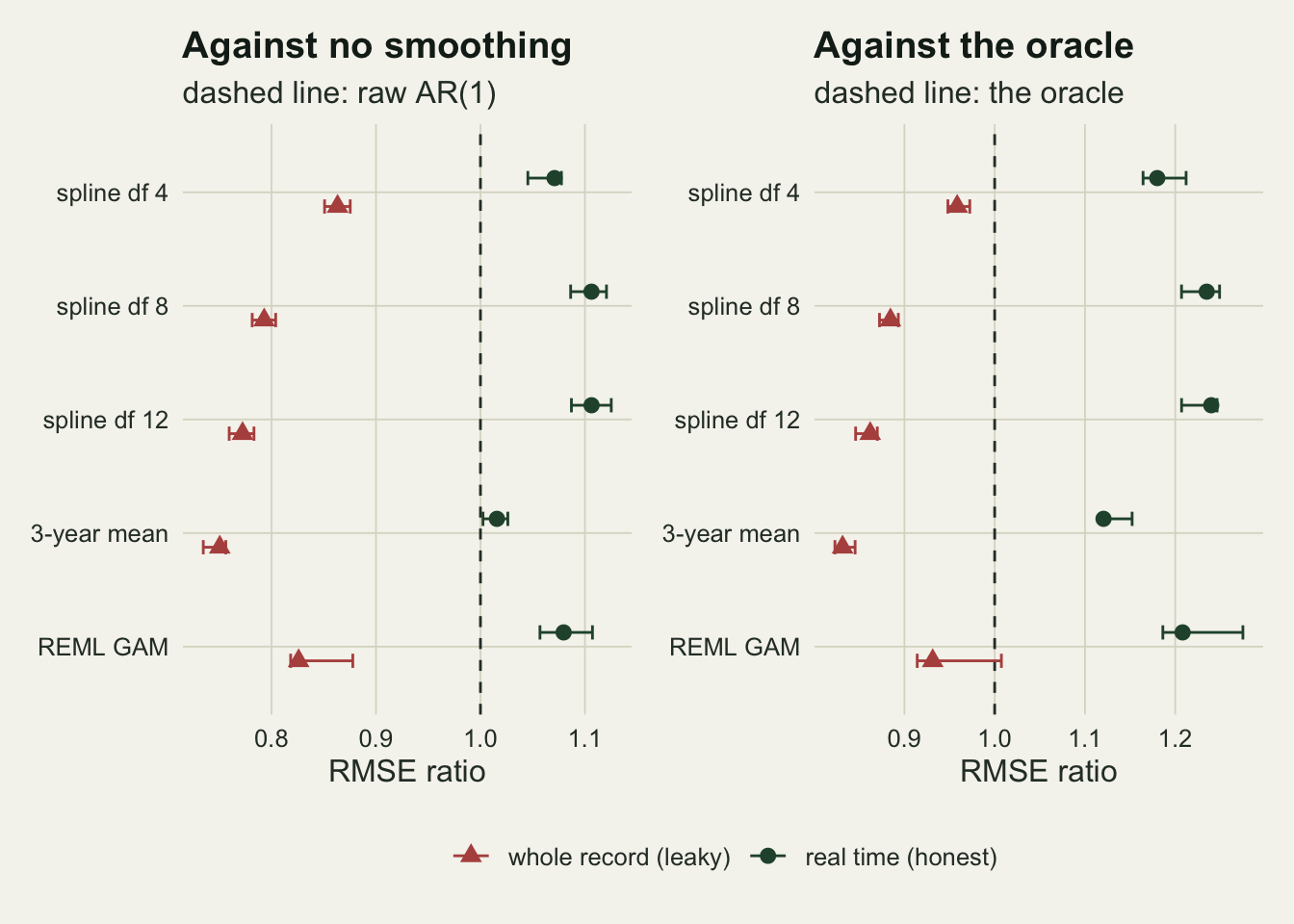

Figure 2: One-step forecast error relative to the raw autoregression (left) and relative to the oracle that knows the true state and coefficient (right), for five smoothers, each used on the whole record and in real time. Points are the median batch, bars the range over five batches.

The oracle is a floor, but not a usable check

The right panel of the figure uses an oracle that knows the true log abundance in the origin year and the true coefficient, and forecasts 0.7 times the state. Its error against the observed index is closed form: next year’s process innovation plus next year’s counting error, so the square root of 0.15 squared plus 0.25 squared, which is 0.292. The simulated oracle scores 0.291 [0.285, 0.294], which checks the code rather than finding anything. No honest forecaster can beat that floor on average, which is the same idea as the measurement noise floor in gap filling a flux time series, there for filling a missing half hour and here for forecasting a year ahead.

The leaky fixed smoothers pass under it: their ratios to the oracle run from 0.832 for the three-year mean to 0.958 for the spline at 4 degrees of freedom. A forecast that beats the floor on average must have seen something it could not have known, and that is tempting to sell as a check anyone can run. It is not a reliable one. The REML GAM, the smoother an ecologist is most likely to use, sits at 0.931 [0.914, 1.007] of the oracle, further under the floor than the spline at 4 degrees of freedom, yet 1 of its 5 batches lands above it; those batches hold 20 series each, against 100 for the splines.

n_single <- 400                        # fixed before the check was run
set.seed(2530)
floor_cf <- sqrt(sd_proc^2 + sd_obs_main^2)
single <- t(vapply(seq_len(n_single), function(i) {
  y <- sim_index(sd_obs_main)$y; ty <- y[origins + 1]
  score <- function(s) sqrt(mean((sapply(origins, function(t) ar_step(s, t)) - ty)^2))
  c(raw = score(y), lk4 = score(spline_fit(y, 4)))
}, c(raw = 0, lk4 = 0)))
share_raw <- mean(single[, "raw"] < floor_cf)
share_lk4 <- mean(single[, "lk4"] < floor_cf)

In a single series the check has little power either way. Over 400 fresh series, each scored on its own fifteen test years against the closed-form floor, the honest raw autoregression lands under the floor in 38 per cent of series, and the leaky spline at 4 degrees of freedom fails to get under it in 33 per cent. And the floor itself needs the process standard deviation, which the reader has to estimate; the Gompertz post shows in its section on why the split is hard that a single series pins down the total variance but not how it divides between process and counting error. The practical check is the one the repair already provides: refit at every origin and look again.

How much of the gain is next year’s counting error

Scoring against the true state instead of the observed index splits the leaky gain. The error of a forecast against the observed value is its error against the true state, minus twice the covariance between that error and next year’s counting error, plus the counting-error variance. For an honest forecast the covariance is zero in expectation, because nothing available at the origin knows next year’s counting error. For a leaky one it is positive. The difference in squared error between raw and leaky arms therefore splits exactly into a part from tracking the state better and a part from reading the target’s own counting error.

sd_obs_grid <- c(0.1, 0.25, 0.4)
set.seed(2610)
L_lo <- lapply(seq_len(n_batch), function(k) run_batch(n_per_batch, 0.1, 12))
set.seed(2640)
L_hi <- lapply(seq_len(n_batch), function(k) run_batch(n_per_batch, 0.4, 12))
cells <- list(L_lo, L_main, L_hi)
split_gain <- function(L, a) {
  m <- Reduce(`+`, L); nn <- m["n", a]
  total <- (m["sy", "raw"] - m["sy", a]) / nn
  state <- (m["sx", "raw"] - m["sx", a]) / nn
  noise <- 2 * (m["cr", a] - m["cr", "raw"]) / nn
  c(total = total, state = state, noise = noise, gap = total - state - noise,
    rel_total = total / (m["sy", "raw"] / nn))
}
sp_df12 <- sapply(cells, split_gain, a = "leaky spline df 12")
sp_ma3  <- sapply(cells, split_gain, a = "leaky 3-year mean")
id_gap <- max(abs(c(sp_df12["gap", ], sp_ma3["gap", ])))
noise_share12 <- sp_df12["noise", ] / sp_df12["total", ]
noise_share3  <- sp_ma3["noise", ] / sp_ma3["total", ]
tab_lo <- cell_long(L_lo); tab_hi <- cell_long(L_hi)
tabs <- list(tab_lo, tab_main, tab_hi)
r12 <- sapply(tabs, function(tb) q3(tb, "leaky spline df 12", "ratio_raw")[1])
r12_rt <- sapply(tabs, function(tb) q3(tb, "real-time spline df 12", "ratio_raw"))
r3_rt <- sapply(tabs, function(tb) q3(tb, "real-time 3-year mean", "ratio_raw"))
sx12 <- sapply(tabs, function(tb) q3(tb, "leaky spline df 12", "rmse_x")[1])
sxraw <- sapply(tabs, function(tb) q3(tb, "raw", "rmse_x")[1])
sxorc <- sapply(tabs, function(tb) q3(tb, "oracle", "rmse_x")[1])
honest_cr <- max(abs(sapply(cells, function(L) { m <- Reduce(`+`, L)
  m["cr", c("raw", "real-time spline df 12", "real-time 3-year mean")] / m["n", 1] })))

The split is an identity in the simulated data, and it closes to within floating-point rounding. For the honest arms the covariance term is at most 0.0022 in absolute value, noise around zero as it should be.

For the spline at 12 degrees of freedom, the share of the apparent gain in squared error that is next year’s counting error read back into its own forecast is 25 per cent at counting error 0.10, 67 per cent at 0.25 and 95 per cent at 0.40. For the centred three-year mean the shares are 32, 74 and 98 per cent. The noisier the counts, the more of the hindcast gain is the counting error of the year being forecast, which is the least useful thing a population forecast could claim to predict.

The rest of the gain is better tracking of the state, and even that is partly borrowed from the future, because the whole-record smooth has also seen part of next year’s process innovation. Against the true state, the leaky spline at 12 degrees of freedom scores 0.128, 0.163 and 0.216 across the three noise levels, against 0.170, 0.206 and 0.224 for the raw autoregression and 0.150, 0.150 and 0.150 for the oracle, whose error against the state is the process standard deviation, 0.15, by construction. At the lowest noise level the leaky spline beats the oracle even against the state, which no forecast made at the origin can do on average.

The reversal holds at every noise level. On the whole record the spline at 12 degrees of freedom has median ratios of 0.743 and 0.802 at the lowest and highest counting error. In real time the spline at 12 degrees of freedom has ratios of 1.061 [1.032, 1.072], 1.106 [1.087, 1.125] and 1.148 [1.120, 1.178] to raw, and the trailing three-year mean 1.070 [1.038, 1.076], 1.016 [1.002, 1.026] and 1.024 [1.020, 1.031].

raw_mse <- sapply(cells, function(L) { m <- Reduce(`+`, L); m["sy", "raw"] / m["n", "raw"] })
split_df <- rbind(
  data.frame(smoother = "leaky spline df 12", sd_obs = sd_obs_grid,
             part = "tracks the true state", val = 100 * sp_df12["state", ] / raw_mse),
  data.frame(smoother = "leaky spline df 12", sd_obs = sd_obs_grid,
             part = "reads next year's counting error", val = 100 * sp_df12["noise", ] / raw_mse),
  data.frame(smoother = "leaky 3-year mean", sd_obs = sd_obs_grid,
             part = "tracks the true state", val = 100 * sp_ma3["state", ] / raw_mse),
  data.frame(smoother = "leaky 3-year mean", sd_obs = sd_obs_grid,
             part = "reads next year's counting error", val = 100 * sp_ma3["noise", ] / raw_mse))
split_df$part <- factor(split_df$part,
                        levels = c("reads next year's counting error", "tracks the true state"))
split_df$smoother <- factor(split_df$smoother, levels = c("leaky spline df 12", "leaky 3-year mean"))
split_df$sd_lab <- factor(sprintf("%.2f", split_df$sd_obs), levels = sprintf("%.2f", sd_obs_grid))
ggplot(split_df, aes(sd_lab, val, fill = part)) +
  geom_col(width = 0.65, colour = te_paper, linewidth = 0.3) +
  facet_wrap(~ smoother) +
  scale_fill_manual(values = c(te_rust, te_forest), name = NULL) +
  labs(x = "standard deviation of the counting error",
       y = "apparent gain, % of raw AR(1) squared error",
       title = "What the leaky hindcast gain is made of",
       subtitle = "each bar is the whole-record smoother's gain over raw AR(1)") +
  theme_datasheet() + theme(legend.position = "bottom",
                            strip.text = element_text(colour = te_ink, face = "bold"))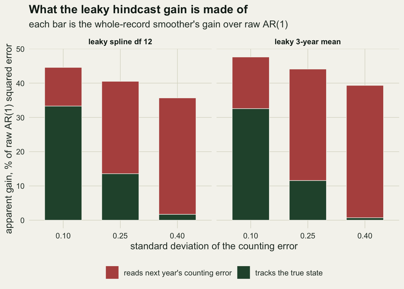

Figure 3: The hindcast gain of two leaky smoothers over the raw autoregression, in squared error as a percentage of the raw error, split into better tracking of the true state and next year’s counting error read back into its own forecast, at three levels of counting error.

Why the honest smoother loses

The obvious explanation is that the endpoint of a smooth is poorly determined, because it has data on one side only. How that plays out for a fitted trend is the business of derivatives of a smooth trend, and the lag it introduces is not the subject here. What the forecast depends on is narrower: how far the value at the origin sits from the true state, and what the autoregression does with it.

ep <- function(tb, a) q3(tb, a, "base_err")[1]
pooled_slopes <- function(L, a) {
  m <- Reduce(`+`, L)[, a]
  c(fitted = unname(m["sl"] / m["n"]),
    best = unname((m["by"] - m["b1"] * m["y1"] / m["n"]) / (m["b2"] - m["b1"]^2 / m["n"])))
}
ep_raw  <- ep(tab_main, "raw")
ep_rt   <- sapply(arm_pairs$realtime, function(a) ep(tab_main, a))
ep_leak <- sapply(arm_pairs$leaky, function(a) ep(tab_main, a))
ep_reml <- c(ep(tab_reml, "leaky REML GAM"), ep(tab_reml, "real-time REML GAM"))
sl_raw  <- pooled_slopes(L_main, "raw")
sl_rt12 <- pooled_slopes(L_main, "real-time spline df 12")
sl_rt3  <- pooled_slopes(L_main, "real-time 3-year mean")
sl_rtg  <- pooled_slopes(L_reml, "real-time REML GAM")
sl_lk12 <- pooled_slopes(L_main, "leaky spline df 12")
set.seed(2560)
long_y <- sim_index(sd_obs_main, 1e5)$y      # one very long series, same model
sl_long <- ar_fit(long_y, length(long_y))[2]

The endpoint turns out not to be the problem. For the raw index the distance from the state is just the counting error, 0.250 in root mean square. The endpoints of the real-time splines sit closer: 0.181, 0.190 and 0.207 at 4, 8 and 12 degrees of freedom, 0.180 for the trailing mean and 0.192 for the real-time GAM. The whole-record smoothers at the same years sit closer still, 0.166, 0.150 and 0.149 for the splines and 0.159 for the GAM. So the real-time smooth does start from a better estimate of this year’s population than the raw index does, and still forecasts next year worse.

The loss is in the slope. The autoregression on the raw index is fitted to 25 to 39 years, and a least-squares autoregressive coefficient from a short series is biased towards zero: its average fitted slope is 0.186, while the slope that would have been best for forecasting from the raw value, found by regressing next year’s index on this year’s across all series and origins, is 0.278. The same fit on one series of 100,000 years gives 0.292, so the gap is the short window; counting error has already pulled both far below the state’s 0.7. That is too shallow, by a factor of 0.67, but a shallow slope errs on the safe side, towards forecasting the mean. The autoregression on a smooth is fitted mostly to interior values of the smooth, which are strongly autocorrelated, and it learns a steep slope: 0.853 on average for the real-time spline at 12 degrees of freedom, where the best slope for forecasting from that spline’s endpoint is 0.338, a factor of 2.53 too steep. For the real-time GAM the two are 0.981 and 0.410, and for the trailing mean 0.734 and 0.407. The coefficient is learned from the smooth’s own persistence from year to year, which the smoothing has pushed above the state’s 0.7, and it is then used to forecast next year’s observed index from the endpoint, so every error left in the endpoint is carried forward with little damping. In the leaky version the value at the origin is an interior value like the ones the slope was learned on, so the mismatch does not arise: the slope fitted there, 0.889, is if anything shallower than its own best value of 1.027, which is above one because the leaky value at the origin already contains part of next year.

If the mismatch is the cause, learning the slope where it is used should remove it. The check below keeps the real-time spline at 12 degrees of freedom but changes the regression: at each origin it regresses next year’s observed index on the real-time endpoint of every earlier year, each endpoint computed from the years up to it, and forecasts from the endpoint at the origin.

k_min <- 15                             # first year with an endpoint; fixed before the run
yon_fit <- function(y, z, t) {          # regress y[k + 1] on z[k] for k < t, forecast from z[t]
  k <- which(is.finite(z[1:(t - 1)])); z0 <- z[k]; z1 <- y[k + 1]
  slope <- sum((z0 - mean(z0)) * (z1 - mean(z1))) / sum((z0 - mean(z0))^2)
  mean(z1) + slope * (z[t] - mean(z0))
}
yon_series <- function() {
  y <- sim_index(sd_obs_main)$y; ty <- y[origins + 1]
  ep12 <- rep(NA_real_, n_year)
  for (k in k_min:max(origins)) ep12[k] <- spline_fit(y[1:k], 12)[k]
  y_k <- ifelse(seq_len(n_year) >= k_min, y, NA)
  fc <- list(raw = sapply(origins, function(t) ar_step(y, t)),
             ep12 = sapply(origins, function(t) yon_fit(y, ep12, t)),
             raw_k = sapply(origins, function(t) yon_fit(y, y_k, t)))
  vapply(fc, function(p) sum((p - ty)^2), 0)
}
set.seed(2550)
Y_ep <- lapply(seq_len(n_batch), function(b)
  Reduce(`+`, lapply(seq_len(n_per_batch), function(i) yon_series())))
yon_ratio <- function(a, ref) {
  v <- vapply(Y_ep, function(m) sqrt(m[[a]] / m[[ref]]), 0); c(median(v), range(v))
}
r_yon_raw  <- yon_ratio("ep12", "raw")
r_yon_same <- yon_ratio("ep12", "raw_k")
r_rawk     <- yon_ratio("raw_k", "raw")   # cost of dropping the years before k_min

The first endpoint is at year 15, so the check is compared both with the usual raw autoregression and with a raw autoregression restricted to the same years. Over 500 new series the endpoint regression has a ratio of 1.027 [1.025, 1.039] to the usual raw autoregression, against 1.106 [1.087, 1.125] for the real-time spline with its slope learned on its own lag. The raw autoregression restricted to those years has a ratio of 1.030 [1.025, 1.039] to the usual one, so what is left of the gap is the early years the check cannot use; against that restricted raw fit the endpoint regression is 0.997 [0.996, 1.000], a tie for practical purposes. The loss came from the pipeline, not from the smoothed value, and repairing the pipeline still leaves the smoother with nothing to add over the raw index.

A filter is the fair real-time smoother

The principled one-sided smoother for this model is the Kalman filter. A first-order autoregression observed with independent error is an ARMA(1,1) process, and arima() computes one-step forecasts of the ARMA(1,1), which contains that model, through a Kalman filter. If any real-time smoothing should help, it is this one.

kalman_prior_var <- function(b, sp, so) {
  P <- sp^2
  for (i in 1:500) P <- b^2 * P * so^2 / (P + so^2) + sp^2
  P
}
var_x <- sd_proc^2 / (1 - b_true^2); var_y <- var_x + sd_obs_main^2
rho1 <- b_true * var_x / var_y
rmse_ar_inf <- sqrt(var_y * (1 - rho1^2))
rmse_kf_inf <- sqrt(kalman_prior_var(b_true, sd_proc, sd_obs_main) + sd_obs_main^2)
rmse_floor  <- sqrt(sd_proc^2 + sd_obs_main^2)
kf_ratio_inf <- rmse_kf_inf / rmse_ar_inf

The ceiling on what it can gain is closed form. With every parameter known and an unlimited series, the best forecast from this year’s index alone is the lag-one autocorrelation of the observed index, 0.290, times this year’s value, with root mean squared error 0.3125. The steady-state Kalman filter, which uses the whole past, reaches 0.3092, and the oracle floor is 0.2915. So the best possible filter improves on the best possible raw autoregression by a ratio of 0.989 at this noise level. The raw autoregression is already close to the best a forecast can do with this series, and that is the other half of why smoothing cannot win here: there is very little to win.

arima_warn <- new.env(); arima_warn$n <- 0
arma_step <- function(y, t) {
  f <- tryCatch(withCallingHandlers(arima(y[1:t], order = c(1, 0, 1), method = "ML"),
                  warning = function(w) { arima_warn$n <- arima_warn$n + 1
                                          invokeRestart("muffleWarning") }),
                error = function(e) NULL)
  if (is.null(f)) return(NA_real_)
  predict(f, n.ahead = 1)$pred[1]
}
filter_series <- function(n_tot, n_tr) {
  d <- sim_index(sd_obs_main, n_tot); y <- d$y; org <- n_tr:(n_tot - 1)
  fcs <- list(raw = sapply(org, function(t) ar_step(y, t)),
              arma = sapply(org, function(t) arma_step(y, t)))
  ty <- y[org + 1]
  sapply(fcs, function(p) c(sy = sum((p - ty)^2, na.rm = TRUE), n = sum(is.finite(p))))
}
filter_batch <- function(n_ser, n_tot, n_tr)
  Reduce(`+`, lapply(seq_len(n_ser), function(i) filter_series(n_tot, n_tr)))
n_per_batch_arma <- 20; n_long <- 100  # fixed before any arm was run
set.seed(2540)
F40 <- lapply(seq_len(n_batch), function(k) filter_batch(n_per_batch_arma, n_year, n_train))
set.seed(2541)
F100 <- lapply(seq_len(n_batch), function(k) filter_batch(n_per_batch_arma, n_long, n_long - 15))
f_ratio <- function(Fl) vapply(Fl, function(m)
  sqrt((m["sy", "arma"] / m["n", "arma"]) / (m["sy", "raw"] / m["n", "raw"])), 0)
fr40 <- f_ratio(F40); fr100 <- f_ratio(F100)
n_fits <- 2 * n_batch * n_per_batch_arma * 15
n_fail <- sum(vapply(c(F40, F100), function(m) 15 * n_per_batch_arma - m["n", "arma"], 0))

In the forty-year series, with the ARMA refitted at every origin, its ratio to the raw autoregression is 1.010 [1.002, 1.018]. In series of 100 years, forecasting the last fifteen, it is 1.003 [0.989, 1.009]. Every one of the fits returned a forecast. arima() gave a convergence warning on 3 of the 3000 fits; those forecasts are kept as they are, since a forecaster running the method would have them too. Of the 5 long-series batches, 2 fall below one; of the short-series batches, 0. The filter does not reliably beat raw at either length, presumably because the gain it could deliver with known parameters is about one per cent and the cost of estimating the extra moving-average parameter from series of this length is of the same size or larger. It never does as badly as the real-time spline or GAM forecasts with the slope learned on the smooth’s own lag either.

fil_df <- data.frame(len = factor(rep(c("40 years", "100 years"), each = n_batch),
                                  levels = c("40 years", "100 years")),
                     ratio = c(fr40, fr100))
rt_ref <- data.frame(y = r_reml_rt[1], lab = "real-time REML GAM, 40 years")
ggplot(fil_df, aes(len, ratio)) +
  geom_hline(yintercept = 1, colour = te_body, linetype = "dashed", linewidth = 0.5) +
  geom_hline(yintercept = kf_ratio_inf, colour = te_gold, linewidth = 0.9) +
  geom_hline(data = rt_ref, aes(yintercept = y), colour = te_rust, linewidth = 0.7,
             linetype = "longdash") +
  geom_point(colour = te_forest, size = 3, position = position_jitter(width = 0.08, height = 0,
                                                                      seed = 1)) +
  annotate("text", x = 0.55, y = kf_ratio_inf, label = "known-parameter filter, unlimited series",
           vjust = 1.6, hjust = 0, colour = te_body, size = 3.3) +
  annotate("text", x = 2.45, y = 1, label = "raw AR(1)", vjust = -0.6, hjust = 1,
           colour = te_body, size = 3.3) +
  annotate("text", x = 2.45, y = r_reml_rt[1], label = "real-time REML GAM, 40 years",
           vjust = -0.6, hjust = 1, colour = te_rust, size = 3.3) +
  labs(x = "series length", y = "RMSE ratio to raw AR(1)",
       title = "A filter ties with raw; the real-time GAM loses",
       subtitle = "green points: ARMA(1,1) refitted at each origin, one per batch") +
  theme_datasheet()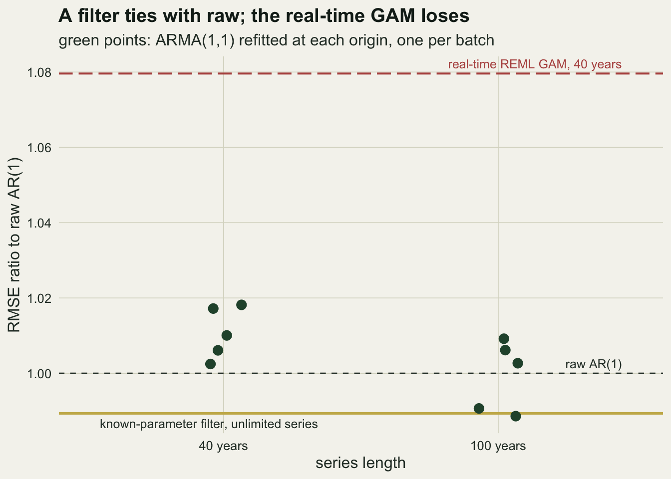

Figure 4: The ARMA(1,1) Kalman forecast relative to the raw autoregression, batch by batch, in forty-year and hundred-year series, against the closed-form ratio the filter would reach with known parameters and an unlimited series.

What to report

Say where the smoothing happened relative to each forecast origin. A hindcast from a smoother fitted to the whole record is not an out-of-sample test, however carefully the origins were rolled forward, and a reader cannot tell the difference from the table of errors alone.

Run the rolling-origin version. Refit every step, the smoother included, on the years before the origin, and forecast from what that fit gives at the origin. It is the same rule as moving preprocessing inside a cross-validation fold, and in a series it can change the conclusion, not just the size of the number. For one-step forecasts of an index like the one simulated here, the honest answer was to drop the smoother.

Score against the observed index and say so. The error of a leak-free forecast against the observed value is its error against the state plus the counting error, so a forecast that beats the closed-form floor on average has seen the future; the converse does not hold: a leaky forecast need not land under it in a given test set (one REML batch did not), and one series is too noisy to tell.

Report the raw autoregression next to any smoothed or filtered method, on the same series and origins, and persistence as well. A smoothing method earns its place by beating raw in the rolling-origin test, not in the whole-record one.

If only a published smoothed index is available, the one-step test cannot be made honest from it, because every value in it was computed with later years. The annual unsmoothed index, or archived releases of the smoothed one as it stood in each year, are the inputs a hindcast needs.

Honest limits

The generating process is a stationary first-order Gompertz model with Gaussian counting error on the log scale. It has no trend, no change point and no cycle, which is the case where a raw autoregression is close to optimal: the closed-form ceiling says a perfect filter gains about one per cent. An index with a long-run trend, or with process dynamics that a smoother captures and a first-order autoregression does not, could give the real-time smoother something to win, and nothing here shows it would not.

The forecast is one step ahead. Smoothed indices are also used for multi-year projections, and for trend estimates rather than forecasts at all. The Fewster rule of three tenths of the series length was designed for describing the shape of a trend, not as an input to a forecast, and none of the numbers above says it is wrong for that purpose. What they say is that an autoregression learned on the interior of a trend smooth does not transfer to its endpoint, which is where a forecast starts.

The degrees of freedom of the real-time splines were held fixed as the window grew, so 12 degrees of freedom on 25 years is a wigglier smooth than 12 on 40. The REML GAM chooses its own smoothness at every origin and lost as well, and the trailing mean, which has no smoothness to choose, lost by 1.6 to 7.0 per cent across the three noise levels, so the reversal does not rest on that choice, but a spline whose degrees of freedom scale with the window was not run.

The autoregression on the smooth is fitted by least squares on the smoothed values, as a practitioner would. A smoothed series is strongly autocorrelated by construction, so that fit learns a slope suited to the interior of the smooth, as the section on why the honest smoother loses showed. Regressing next year’s index on the real-time endpoint, instead of the smooth on its own lag, removes the loss, but it only ties a raw autoregression fitted to the same years, just as the filter only ties raw: smoothing gains nothing here either way.

Bergmeir, Hyndman and Koo show that ordinary cross-validation is valid for purely autoregressive prediction when the errors are uncorrelated, so the problem here is not that folds were not blocked in time. It is a preprocessing step that used the future before any fold or origin existed, and it would break a blocked or rolling design just as surely. Ward and colleagues found across thousands of vertebrate population series that simple low-dimensional models gave the most accurate short-term forecasts, and that repeating the last observation rivalled more elaborate methods; the raw autoregression winning here is in line with that, but one simulated process is not a survey.

References

Tashman LJ 2000 International Journal of Forecasting 16(4):437-450 (10.1016/S0169-2070(00)00065-0)

Fewster RM, Buckland ST, Siriwardena GM, Baillie SR, Wilson JD 2000 Ecology 81(7):1970-1984 (10.1890/0012-9658(2000)081[1970:AOPTFF]2.0.CO;2)

Bergmeir C, Hyndman RJ, Koo B 2018 Computational Statistics and Data Analysis 120:70-83 (10.1016/j.csda.2017.11.003)

Ward EJ, Holmes EE, Thorson JT, Collen B 2014 Oikos 123(6):652-661 (10.1111/j.1600-0706.2014.00916.x)

Related tutorials

• Data leakage in ecological model validation
• Forecast skill and the baseline
• Gompertz state-space model in R
• Simplex projection and delay embedding