library(ggplot2)

te_pal <- list(forest = "#275139", green = "#2f8f63", sage = "#93a87f",
               clay = "#b5534e", gold = "#cda23f", line = "#dad9ca",
               ink = "#16241d", paper = "#f5f4ee")

theme_te <- function() {
  theme_minimal(base_size = 12) +
    theme(panel.grid.minor = element_blank(),
          panel.grid.major = element_line(colour = "#e7e6dc"),
          plot.background = element_rect(fill = "#f5f4ee", colour = NA),
          panel.background = element_rect(fill = "#f5f4ee", colour = NA),
          plot.title = element_text(face = "bold", colour = te_pal$ink),
          axis.title = element_text(colour = "#2c3a31"),
          axis.text = element_text(colour = "#2c3a31"))
}Gap filling a flux time series
R
missing data
time series
carbon flux
ecology tutorial
Eddy covariance gap filling in R: three missing-data mechanisms in a year of half-hourly net ecosystem exchange, five fills scored against a known budget.
A flux tower stands over a mixed forest, logging a three-dimensional sonic anemometer and an infrared gas analyser at ten hertz and writing out one covariance every thirty minutes. A calendar year of that is seventeen and a half thousand numbers, each of them a net ecosystem exchange of carbon dioxide in micromoles per square metre per second, negative when the canopy takes carbon up and positive when it gives carbon back. The site is asked for one figure at the end of the year: how much carbon the forest gained or lost, in gC/m2/yr.
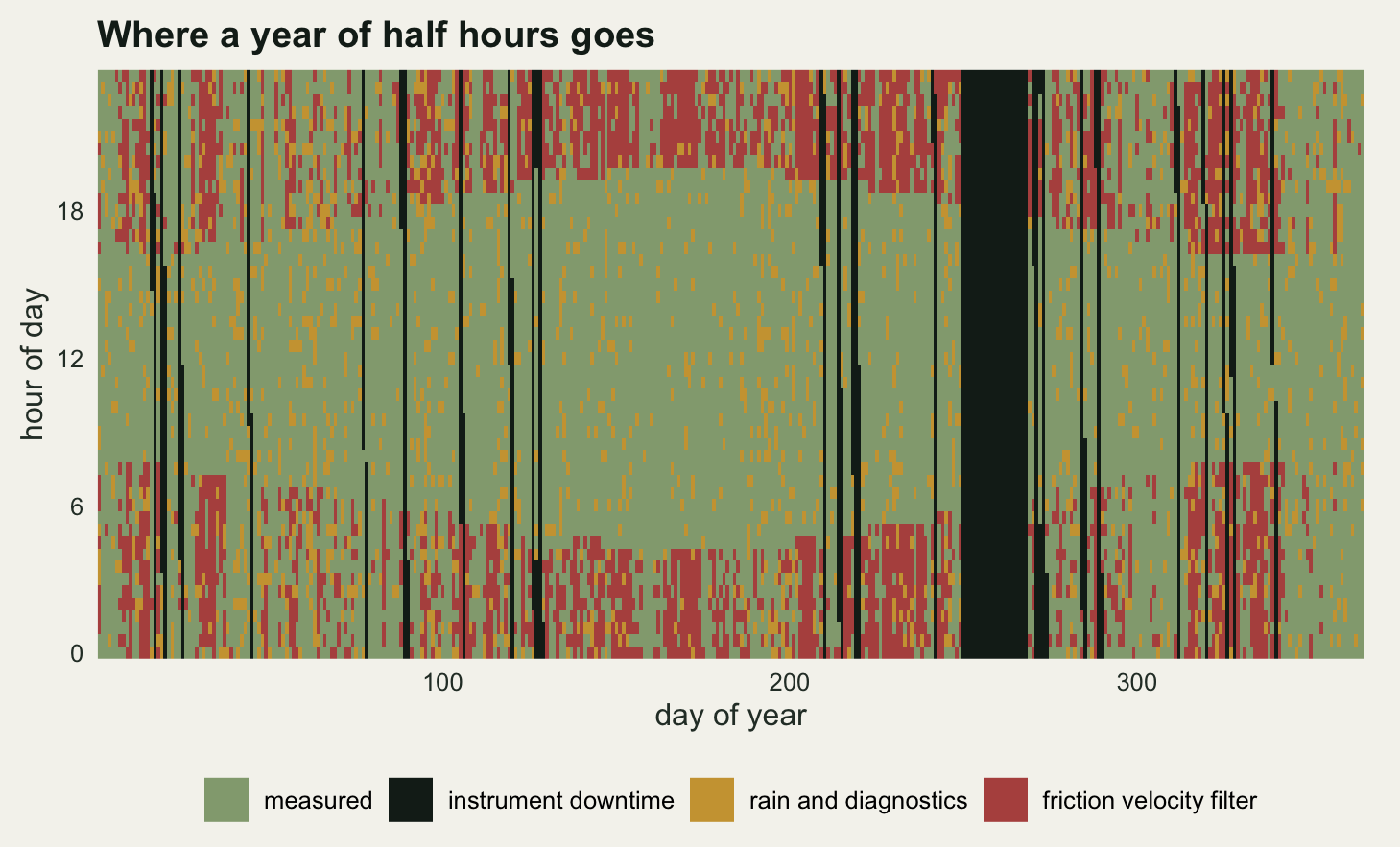
That figure is a sum over every half hour of the year, and the tower did not deliver every half hour. Some are gone because the mains failed and the analyser was cold for a day and a half. Some are gone because it rained on the sonic and the diagnostic flag went up. Some are gone because the analyst deleted them on purpose: on calm nights the eddy covariance method undercounts, so half hours with a friction velocity below a site-specific threshold are thrown out as a matter of protocol. Published towers report thirty to forty-five per cent of half hours missing in a typical year, and the annual sum has to be produced anyway.
The gap-filling literature starts from that arithmetic. Falge et al (2001) put the problem in its modern form, comparing fills across a network of sites and showing that the choice of method moves the published annual sum; Reichstein et al (2005) supplied the look-alike matching algorithm most towers now run; Moffat et al (2007) benchmarked fifteen techniques against artificial gaps. What all three keep saying, and what is easy to lose in the software, is that the damage is not proportional to how much is missing. This post measures that on a simulated year where the true flux is known at every half hour, three mechanisms remove half hours in three patterns, and five filling methods compete on two scores at once: the point-level root mean squared error at the gaps, and the annual sum against the truth.
It sits next to the missing-data cluster and does not repeat it. Single imputation: bias and variance works on a rectangular dataset with a missing response, and the quantity at stake is a regression slope; multiple imputation by chained equations fixes the uncertainty single imputation hides, again for a slope. Two things change here. The quantity is a total over the same rows being filled, so a bias of a fraction of a micromole in a typical half hour arrives in the answer multiplied by the length of the year. And the missingness is manufactured by the measurement system rather than by nature: one mechanism per cause, each with its own relationship to the flux, sorted by the taxonomy of Rubin (1976) that missing data: MCAR, MAR and MNAR covers from the general side.
Three sibling posts carry the parts this one leaves alone. Night-time flux and the u-star threshold is where the friction velocity threshold comes from; here it is simply assumed to exist. Partitioning net flux into GPP and respiration takes the filled series apart afterwards, and checking an annual flux budget asks whether the finished number is defensible.
A year the simulation knows exactly
The drivers come first, because every fill below leans on them. Global radiation follows clear-sky solar geometry at forty-seven degrees north, dimmed by a cloudiness series with a synoptic persistence of a day or two. Air temperature carries a seasonal cycle, a diurnal cycle whose amplitude grows in summer, and a slow weather departure. Vapour pressure deficit is computed from air temperature and a relative humidity that falls when the sun is out and the air is warm.
n_day <- 365
n_hh  <- 48
n_tot <- n_day * n_hh
doy   <- rep(seq_len(n_day), each = n_hh)
hod   <- rep(seq(0, 23.5, by = 0.5), times = n_day)
conv_gc <- 12.011e-6 * 1800        # umol/m2/s for half an hour -> gC/m2

lat_rad  <- 47 * pi / 180
decl     <- 23.45 * pi / 180 * sin(2 * pi * (284 + doy) / 365)
hour_ang <- (hod - 12) * 15 * pi / 180
cos_zen  <- sin(lat_rad) * sin(decl) + cos(lat_rad) * cos(decl) * cos(hour_ang)
rg_pot   <- 1000 * pmax(cos_zen, 0)
is_night <- rg_pot < 20

ar1 <- function(nn, phi, sdv) {
  as.numeric(stats::filter(rnorm(nn, 0, sdv), phi, method = "recursive"))
}

set.seed(20260802)
cloud_z   <- ar1(n_tot, 0.988, 1)
cloud_z   <- cloud_z / sd(cloud_z)
clearness <- 0.32 + 0.62 * plogis(1.1 * cloud_z)
rg        <- rg_pot * clearness

ta_seas <- 9.5 + 10.5 * sin(2 * pi * (doy - 111) / 365)
ta_diur <- (4 + 2.2 * sin(2 * pi * (doy - 111) / 365)) * sin(2 * pi * (hod - 9) / 24)
ta      <- ta_seas + ta_diur + ar1(n_tot, 0.985, 0.42)

es_kpa <- 0.6108 * exp(17.27 * ta / (ta + 237.3))
rh     <- 0.93 - 0.30 * (rg / 900) - 0.011 * (ta - 9.5) + ar1(n_tot, 0.97, 0.012)
rh     <- pmin(pmax(rh, 0.22), 0.99)
vpd    <- 10 * es_kpa * (1 - rh)

print(round(c(half_hours = n_tot, night_share = mean(is_night),
              max_rg = max(rg), mean_daytime_rg = mean(rg[!is_night]),
              min_ta = min(ta), max_ta = max(ta), mean_ta = mean(ta),
              max_vpd = max(vpd), mean_vpd = mean(vpd)), 3))
half_hours night_share max_rg mean_daytime_rg min_ta
17520.000 0.508 815.903 280.584 -10.465
max_ta mean_ta max_vpd mean_vpd
32.306 9.409 22.906 2.590 The year holds 17520 half hours, 50.82 per cent of them dark, with radiation peaking at 816 W/m2, air temperature running from -10.46 to 32.31 degrees C, and vapour pressure deficit reaching 22.91 hPa on the driest summer afternoons.
The flux itself is built from two processes that every partitioning scheme assumes. Gross primary production follows a saturating light response scaled by a phenology curve and throttled at high vapour pressure deficit. Ecosystem respiration follows the Lloyd and Taylor temperature function with a small phenological term on top. Net ecosystem exchange is respiration minus production, so it is negative when the canopy is winning.
On top of that goes measurement noise. Richardson et al (2006) measured the random error of half-hourly tower fluxes at eight sites and found two things that a simulation has to carry: the error scales with the size of the flux, and its distribution is double exponential rather than normal, with heavier tails than a Gaussian of the same width.
lai_f   <- plogis((doy - 118) / 9) * plogis((298 - doy) / 11)
alpha_q <- 0.055
gpp_max <- 40
f_vpd   <- exp(-0.035 * pmax(vpd - 8, 0))
gpp     <- lai_f * f_vpd * (alpha_q * rg * gpp_max) / (alpha_q * rg + gpp_max)

r_ref <- 2.0
e0    <- 230
reco  <- r_ref * exp(e0 * (1 / (283.15 - 227.13) - 1 / (ta + 273.15 - 227.13))) *
  (0.7 + 0.5 * lai_f)
nee_true <- reco - gpp

set.seed(4102026)
sig_v <- 0.50 + 0.16 * abs(nee_true)
nee_m <- nee_true + sig_v * (rexp(n_tot) - rexp(n_tot)) / sqrt(2)
eps   <- nee_m - nee_true

truth_annual <- sum(nee_m) * conv_gc
noiseless_annual <- sum(nee_true) * conv_gc
print(round(c(max_gpp = max(gpp), max_reco = max(reco),
              mean_nee = mean(nee_true), mean_night_nee = mean(nee_true[is_night]),
              gpp_annual = sum(gpp) * conv_gc, reco_annual = sum(reco) * conv_gc,
              nee_annual_noiseless = noiseless_annual,
              nee_annual = truth_annual), 3))
max_gpp max_reco mean_nee
20.461 7.726 -0.888
mean_night_nee gpp_annual reco_annual
1.680 1180.451 844.027
nee_annual_noiseless nee_annual
-336.424 -338.902 print(round(c(mean_sigma = mean(sig_v), sigma_night = mean(sig_v[is_night]),
sigma_day = mean(sig_v[!is_night]), sd_eps = sd(eps)), 3)) mean_sigma sigma_night sigma_day sd_eps
0.967 0.769 1.171 1.082 Gross primary production peaks at 20.46 umol/m2/s and totals 1180 gC/m2/yr, respiration totals 844 gC/m2/yr, and the difference is an annual net exchange of -338.9 gC/m2/yr. That is the number every method below is trying to recover, and it is a sink of the size a mid-latitude forest reports. Nights average 1.68 umol/m2/s, a steady positive release; the year as a whole averages -0.888.
The measurement noise has a standard deviation of 0.769 umol/m2/s at night and 1.171 in daylight. It is symmetric, so over a whole year most of it cancels: the noiseless annual sum is -336.42 gC/m2/yr and the noisy one -338.9, a difference of 2.48 grams. That is the reason the annual sum is worth computing at all, and it is also why a bias, which does not cancel, is the thing to watch.
Three ways to lose a half hour
The three mechanisms are written separately because they behave separately, and the point of the post is that they are not interchangeable.
Instrument downtime is a power cut, a full disc, a laptop that rebooted, an analyser sent away for repair. It knows nothing about the flux or the weather, and it removes runs rather than isolated half hours. Twenty-six short outages are scattered uniformly through the year, plus one nineteen-day block in early September when the analyser goes off site.
Rain and diagnostics removes half hours through the weather. Rain on the sonic transducer makes the wind measurement unusable, and the analyser’s own flags fire when the optical path is dirty or the sample cell ices up. The probability of loss depends on cloudiness and on air temperature, both of which also drive the flux, so this loss is missing at random given the drivers.
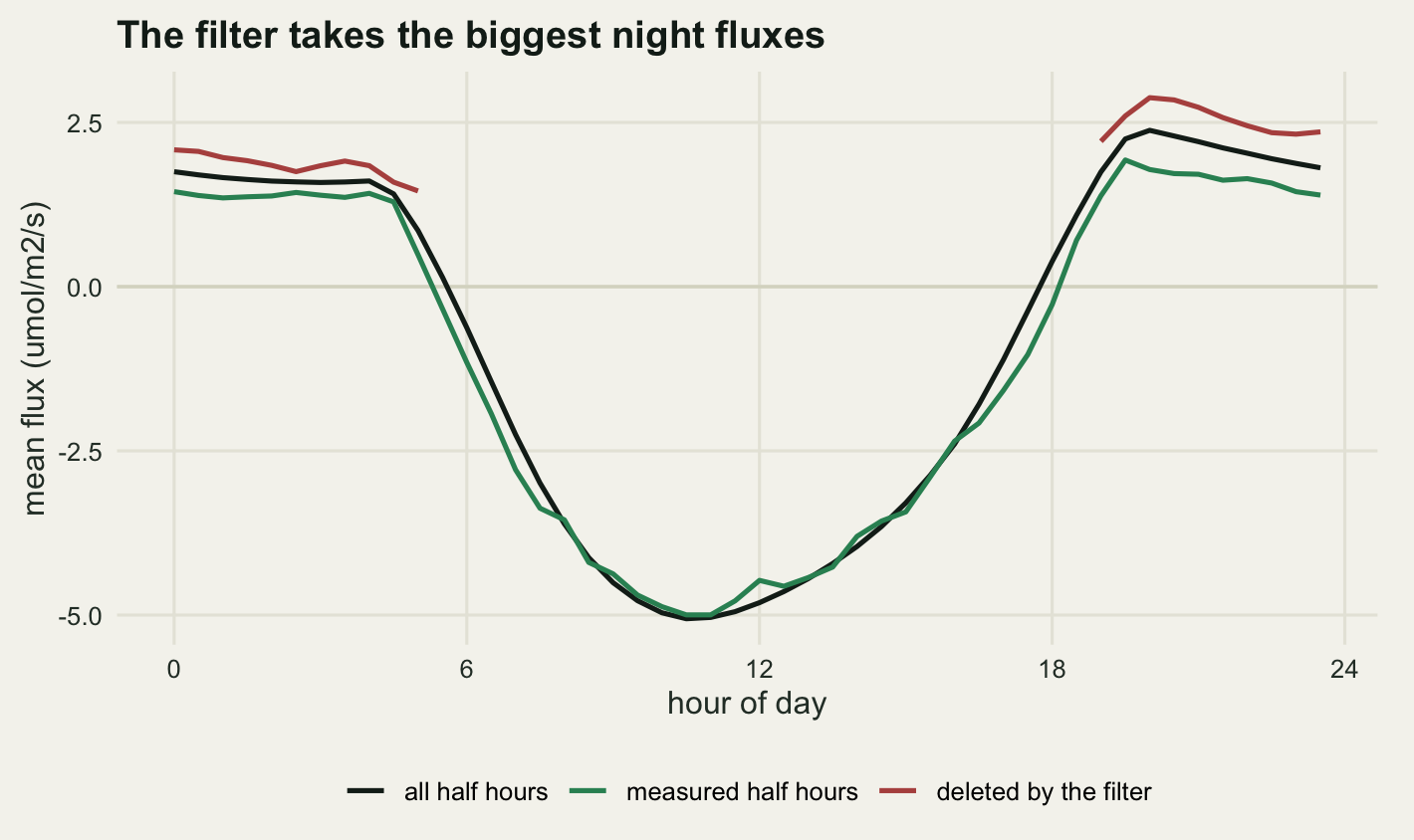
Friction velocity filtering is different in kind, because the analyst does it on purpose. When the air above the canopy is calm, the eddies that carry the flux past the sensor are too weak to be measured, so half hours below a threshold friction velocity are deleted. That threshold is estimated per site and per season; where it comes from is the subject of the u-star threshold post, and here it is fixed at a plausible value. Calm air happens at night, and it happens most on warm, still summer nights, which are exactly the nights when the soil is warm and respiration is at its strongest. The filter therefore removes half hours whose flux value is systematically higher than that of the half hours it leaves behind: missing not at random with respect to the quantity being measured.
set.seed(7112026)
wind_z <- ar1(n_tot, 0.985, 1); wind_z <- wind_z / sd(wind_z)
ustar  <- exp(-1.30 + 0.45 * wind_z + 0.55 * (rg / 900) -
                0.030 * pmax(ta, 0) * is_night + rnorm(n_tot, 0, 0.28))
ustar_thr <- 0.2

## 1: instrument downtime, blocky and indifferent to everything
set.seed(8112026)
n_out  <- 26
out_st <- sample.int(n_tot, n_out)
out_ln <- 10 + rpois(n_out, 46)
m_down <- rep(FALSE, n_tot)
for (k in seq_len(n_out)) {
  m_down[out_st[k]:min(n_tot, out_st[k] + out_ln[k] - 1)] <- TRUE
}
long_start <- (250 - 1) * 48 + 1
long_len   <- 19 * 48
long_idx   <- long_start:(long_start + long_len - 1)
m_down[long_idx] <- TRUE

## 2: rain and diagnostic flags, driven by cloudiness and temperature
set.seed(9112026)
p_rain <- plogis(-1.75 - 5.5 * (clearness - 0.5))
p_diag <- plogis(-4.3 + 0.16 * pmax(-ta, 0))
m_wx   <- (runif(n_tot) < p_rain) | (runif(n_tot) < p_diag)

## 3: the friction velocity filter, applied to night half hours only
m_us <- is_night & ustar < ustar_thr

miss  <- m_down | m_wx | m_us
obs   <- !miss
gaps  <- which(miss)
n_gap <- length(gaps)

print(round(c(downtime = mean(m_down), weather = mean(m_wx),
              ustar_filter = mean(m_us), any_gap = mean(miss),
              downtime_only = mean(m_down & !m_wx & !m_us),
              weather_only = mean(m_wx & !m_down & !m_us),
              ustar_only = mean(m_us & !m_down & !m_wx)), 4))
downtime weather ustar_filter any_gap downtime_only
0.1307 0.1160 0.2167 0.3930 0.0842
weather_only ustar_only
0.0817 0.1604 Coverage lands where a real tower’s does. Downtime touches 13.07 per cent of half hours, weather and diagnostics 11.6 per cent, the friction velocity filter 21.67 per cent, and the union is 39.3 per cent, or 6886 half hours out of 17520. The mechanisms overlap, so the shares do not add: 8.42 per cent is downtime alone, 8.17 per cent weather alone and 16.04 per cent the filter alone.
night_kept <- is_night & obs
print(round(c(night_removed_by_filter = mean(m_us[is_night]),
              mean_flux_kept = mean(nee_true[obs]),
              mean_flux_lost = mean(nee_true[miss]),
              mean_flux_all = mean(nee_true)), 4))
night_removed_by_filter mean_flux_kept mean_flux_lost
0.4264 -1.7133 0.3861
mean_flux_all
-0.8882 print(round(c(night_kept_flux = mean(nee_true[night_kept]),
night_filtered_flux = mean(nee_true[m_us]),
night_all_flux = mean(nee_true[is_night]),
night_kept_temp = mean(ta[night_kept]),
night_filtered_temp = mean(ta[m_us])), 4)) night_kept_flux night_filtered_flux night_all_flux night_kept_temp
1.3467 2.0565 1.6796 4.6151
night_filtered_temp
8.4518 print(round(c(downtime_flux = mean(nee_true[m_down]),
weather_flux = mean(nee_true[m_wx])), 4))downtime_flux weather_flux
-0.9726 -0.4670 runs <- rle(miss)
run_len <- runs$lengths[runs$values]
print(round(c(n_runs = length(run_len), median_run = median(run_len),
mean_run = mean(run_len), longest_run_days = max(run_len) / 48,
share_in_runs_over_a_day = sum(run_len[run_len > 48]) / sum(run_len)), 3)) n_runs median_run mean_run
1952.000 1.000 3.528
longest_run_days share_in_runs_over_a_day
19.125 0.329 The filter removes 42.64 per cent of all night half hours, and the half hours it removes are not a random sample of the night. Their mean true flux is 2.057 umol/m2/s against 1.347 for the night half hours that survive, because the calm nights are the warm ones: mean air temperature 8.45 degrees C in the deleted half hours against 4.62 in the kept ones. That gap of 0.71 umol/m2/s inside the night is the whole story of the post, and it is invisible in any summary of the data that survives.
The other two mechanisms are much better behaved. Half hours lost to downtime average -0.973 umol/m2/s and half hours lost to weather -0.467, both within a micromole of the year’s mean of -0.888. Put the three together and what survives averages -1.713, nearly twice the true mean.
The gaps are also structured in length. There are 1952 separate runs with a median of 1 half hour, but the longest is 19.12 days and 32.88 per cent of all missing half hours sit inside runs longer than a day. Isolated half hours and multi-day blocks are different problems, and Richardson and Hollinger (2007) showed that long gaps carry an uncertainty of their own that short ones do not.
Five fills
The five candidates run on the same masked series. The first is not a filling method at all: take the mean of the half hours that were measured and multiply by the number of half hours in the year, which is what every field campaign reporting a seasonal total from partial coverage has done, usually without saying so. The second is overall mean imputation, the method single imputation: bias and variance opens with, and it puts the same number in every gap. The third is a mean diurnal course computed in a moving window: for a gap in the small hours of a July night, average all the measured values from the same clock time within a week either side, widening the window if none survive. That is the look-up table approach, and it is what most towers ran before the current algorithm arrived. The fourth is linear interpolation between the last measured value before the gap and the first after it.
The fifth is marginal distribution sampling in the sense of Reichstein et al (2005): look for half hours in a moving window whose radiation, temperature and vapour pressure deficit all match the gap’s within tolerances, and average their fluxes. When no such half hour exists, the algorithm falls back through a fixed ladder of weaker conditions, and reporting how often each rung is used is part of using it honestly.
## tolerances and window lengths shared by the last two methods
tol_rg_day   <- 50      # W/m2 on global radiation
tol_rg_night <- 20      # W/m2 when the gap itself is dark
tol_ta       <- 2.5     # degrees C on air temperature
tol_vpd      <- 5       # hPa on vapour pressure deficit
win_short    <- 7L      # days
win_long     <- 14L
win_max      <- 140L

mdc_fill <- function(y_in, ok_v, gaps_v,
                     wins = c(win_short, win_long, 28L, 56L, win_max)) {
  nn <- length(y_in)
  out <- numeric(length(gaps_v))
  for (k in seq_along(gaps_v)) {
    i <- gaps_v[k]
    got <- FALSE
    for (w in wins) {
      jj <- i + 48L * (-w:w)
      jj <- jj[jj >= 1L & jj <= nn]
      jj <- jj[ok_v[jj]]
      if (length(jj)) { out[k] <- mean(y_in[jj]); got <- TRUE; break }
    }
    if (!got) out[k] <- mean(y_in[ok_v])
  }
  out
}
The look-alike matcher is longer because the fallback ladder is the method. Rung A asks for all three drivers within tolerance inside a window of 7 days either side, then the same inside 14 days. Rung B drops temperature and vapour pressure deficit and matches on radiation alone. Rung C abandons the drivers and takes the mean diurnal course within one day, plus or minus an hour. Rung D reruns rung A’s three-driver test on windows widening to 140 days, and rung E does the same for rung C’s mean diurnal course; the radiation-only rung B is never widened. The tolerances are those of the published algorithm: 50 W/m2 on radiation, 20 W/m2 when the gap itself is dark, 2.5 degrees C on air temperature and 5 hPa on vapour pressure deficit.
mds_fill <- function(y_in, ok_v, rg_v, ta_v, vpd_v, hod_v, gaps_v) {
  nn <- length(y_in)
  out <- numeric(length(gaps_v))
  tier <- integer(length(gaps_v))
  gmean <- mean(y_in[ok_v])
  win_a <- c(win_short, win_long)
  win_wide <- c(21L, 28L, 42L, 56L, 84L, win_max)
  win_mdc <- c(2L, 4L, win_short, win_long, 28L, 56L, win_max)
  for (k in seq_along(gaps_v)) {
    i <- gaps_v[k]
    tol_rg <- if (rg_v[i] < tol_rg_day) tol_rg_night else tol_rg_day
    val <- NA_real_
    tt <- 0L
    ## A: all three drivers, the short then the long window
    for (jj in seq_along(win_a)) {
      w <- win_a[jj] * 48L
      cand <- max(1L, i - w):min(nn, i + w)
      okc <- ok_v[cand] & abs(rg_v[cand] - rg_v[i]) <= tol_rg &
        abs(ta_v[cand] - ta_v[i]) <= tol_ta & abs(vpd_v[cand] - vpd_v[i]) <= tol_vpd
      if (any(okc)) { val <- mean(y_in[cand[okc]]); tt <- jj; break }
    }
    ## B: radiation alone, short window
    if (is.na(val)) {
      w <- win_short * 48L
      cand <- max(1L, i - w):min(nn, i + w)
      okc <- ok_v[cand] & abs(rg_v[cand] - rg_v[i]) <= tol_rg
      if (any(okc)) { val <- mean(y_in[cand[okc]]); tt <- 3L }
    }
    ## C: mean diurnal course within one day, plus or minus an hour
    if (is.na(val)) {
      cand <- max(1L, i - 50L):min(nn, i + 50L)
      dh <- abs(hod_v[cand] - hod_v[i])
      okc <- ok_v[cand] & (dh <= 1 | dh >= 23)
      if (any(okc)) { val <- mean(y_in[cand[okc]]); tt <- 4L }
    }
    ## D: all three drivers, windows widening to the maximum
    if (is.na(val)) for (w0 in win_wide) {
      w <- w0 * 48L
      cand <- max(1L, i - w):min(nn, i + w)
      okc <- ok_v[cand] & abs(rg_v[cand] - rg_v[i]) <= tol_rg &
        abs(ta_v[cand] - ta_v[i]) <= tol_ta & abs(vpd_v[cand] - vpd_v[i]) <= tol_vpd
      if (any(okc)) { val <- mean(y_in[cand[okc]]); tt <- 5L; break }
    }
    ## E: mean diurnal course, windows widening to the maximum
    if (is.na(val)) for (w0 in win_mdc) {
      w <- w0 * 48L
      cand <- max(1L, i - w):min(nn, i + w)
      dh <- abs(hod_v[cand] - hod_v[i])
      okc <- ok_v[cand] & (dh <= 1 | dh >= 23)
      if (any(okc)) { val <- mean(y_in[cand[okc]]); tt <- 6L; break }
    }
    if (is.na(val)) { val <- gmean; tt <- 7L }
    out[k] <- val
    tier[k] <- tt
  }
  list(value = out, tier = tier)
}

mds <- mds_fill(nee_m, obs, rg, ta, vpd, hod, gaps)
tier_pct <- 100 * tabulate(mds$tier, 7) / n_gap
names(tier_pct) <- c("A_7d", "A_14d", "Rg_only", "diurnal_1d",
                     "A_widened", "diurnal_widened", "series_mean")
print(round(tier_pct, 3))
A_7d A_14d Rg_only diurnal_1d A_widened
94.148 5.199 0.363 0.029 0.261
diurnal_widened series_mean
0.000 0.000 The ladder is barely used. Rung A at 7 days settles 94.15 per cent of the gaps, the 14 -day version another 5.2 per cent, and everything below that accounts for 0.65 per cent. The last two rungs never fire at all. That is a consequence of an assumption made here for clarity and violated by every real dataset: the drivers are complete. At a real tower the radiation sensor and the thermometer have their own gaps, often at the same moment as the flux, and the deeper rungs exist for exactly that. The 0.26 per cent that does reach rung D sits inside the nineteen-day outage. Measured half hours survive within 14 days of those gaps, but none of them matches all three drivers at once, none matches radiation alone inside the 7 days rung B is allowed, and rung C finds nothing at the same clock time within a day.
fill_mean <- nee_m; fill_mean[miss] <- mean(nee_m[obs])
fill_mdc  <- nee_m; fill_mdc[miss]  <- mdc_fill(nee_m, obs, gaps)
fill_lin  <- approx(which(obs), nee_m[obs], xout = seq_len(n_tot), rule = 2)$y
fill_mds  <- nee_m; fill_mds[miss]  <- mds$value
ann_drop  <- mean(nee_m[obs]) * n_tot * conv_gc
print(round(c(scaled_up_mean = ann_drop,
              overall_mean_fill = sum(fill_mean) * conv_gc), 4))
scaled_up_mean overall_mean_fill
-652.6644 -652.6644 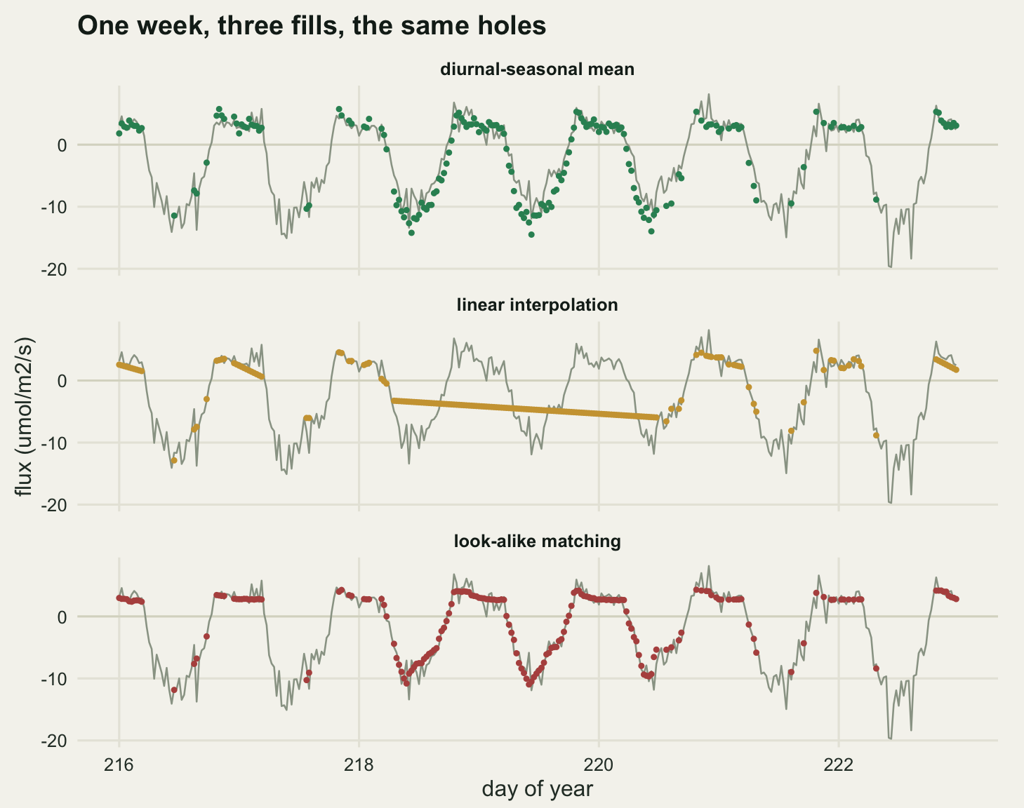
The noise floor, and what beating it would mean
Two scores, computed on the same objects. The point-level score is the root mean squared error between the filled value and the value the instrument actually recorded at that half hour, over the 6886 gap half hours. The annual score is the filled series summed and converted, against the truth.
Before reading either, the floor has to be set. No filling method can predict the measurement noise, because the noise is not a function of anything: the best conceivable predictor of a missing half hour is its own noise-free true flux, and even that leaves the noise behind. The root mean squared error of that ideal predictor is the smallest number any method could report.
floor_rmse <- sqrt(mean(eps[miss]^2))

score_of <- function(v, nm) {
  rm <- sqrt(mean((v[miss] - nee_m[miss])^2))
  data.frame(method = nm, rmse = rm, floor_ratio = rm / floor_rmse,
             annual = sum(v) * conv_gc, error = sum(v) * conv_gc - truth_annual)
}
sc <- rbind(
  data.frame(method = "measured mean scaled up", rmse = NA_real_,
             floor_ratio = NA_real_, annual = ann_drop,
             error = ann_drop - truth_annual),
  score_of(fill_mean, "overall mean fill"),
  score_of(fill_mdc, "diurnal-seasonal mean"),
  score_of(fill_lin, "linear interpolation"),
  score_of(fill_mds, "look-alike matching"))
print(sc$method)
[1] "measured mean scaled up" "overall mean fill"
[3] "diurnal-seasonal mean" "linear interpolation"
[5] "look-alike matching" print(round(sc[, -1], 4)) rmse floor_ratio annual error
1 NA NA -652.6644 -313.7623
2 4.3095 4.3560 -652.6644 -313.7623
3 1.4593 1.4750 -355.1445 -16.2424
4 3.4097 3.4465 -281.4295 57.4725
5 1.0677 1.0792 -341.5161 -2.6140print(round(c(truth = truth_annual, noise_floor = floor_rmse,
lookalike_own_error =
sqrt(sc$rmse[5]^2 - floor_rmse^2)), 4)) truth noise_floor lookalike_own_error
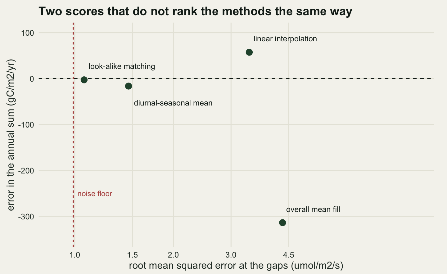
-338.9021 0.9893 0.4016 The floor is 0.9893 umol/m2/s. Look-alike matching reaches 1.0677, which is 1.0792 times the floor: subtract the noise in quadrature and the method’s own error is 0.4016 umol/m2/s, about two fifths of the noise it is swimming in. That is what a method at the floor looks like, and it means the drivers have been used up. Nothing further can be squeezed out of radiation, temperature and vapour pressure deficit at this site; the remaining error is the instrument’s.
The diurnal-seasonal mean sits at 1.4593, or 1.475 times the floor. Linear interpolation reaches 3.4097 and overall mean imputation 4.3095, 4.356 times the floor, which is the number you get for using no information at all.
The first two rows of the annual column are worth staring at. Scaling up the measured mean gives -652.66 gC/m2/yr and filling every gap with the overall mean gives -652.66, and those are not similar numbers, they are the same number to every digit. Filling a gap with the mean of what you measured and then summing is algebraically identical to summing what you measured and multiplying by the ratio of lengths. The field campaign that scales up its measured mean has performed mean imputation without knowing it, and it inherits every property mean imputation has.
Against a truth of -338.9 gC/m2/yr, that number is -313.76 gC/m2/yr out. The forest is reported as taking up about twice as much carbon as it did.
Root mean squared error and the annual sum are different questions
The scatter above is not a diagonal line, and the departures from one are instructive.
in_long <- rep(FALSE, n_tot)
in_long[long_idx] <- TRUE
short_gap <- miss & !in_long

part_of <- function(v, nm) data.frame(
  method = nm,
  rmse_short = sqrt(mean((v[short_gap] - nee_m[short_gap])^2)),
  gC_short = sum(v[short_gap] - nee_m[short_gap]) * conv_gc,
  gC_outage = sum(v[in_long] - nee_m[in_long]) * conv_gc)
parts <- rbind(part_of(fill_mdc, "diurnal-seasonal mean"),
               part_of(fill_lin, "linear interpolation"),
               part_of(fill_mds, "look-alike matching"))
print(parts$method)
[1] "diurnal-seasonal mean" "linear interpolation" "look-alike matching" print(round(parts[, -1], 4)) rmse_short gC_short gC_outage
1 1.2926 -20.2274 3.9850
2 2.3955 -21.6199 79.0924
3 0.9507 -5.2055 2.5915print(round(c(mean_fill_rmse_ratio = sc$floor_ratio[2],
linear_rmse_ratio = sc$floor_ratio[4],
mean_fill_annual_error = sc$error[2],
linear_annual_error = sc$error[4]), 3)) mean_fill_rmse_ratio linear_rmse_ratio mean_fill_annual_error
4.356 3.446 -313.762
linear_annual_error
57.473 Take the two worst point-level performers first. Overall mean imputation has a root mean squared error of 4.31 and linear interpolation 3.41, a difference of only 26.39 per cent. Their annual errors are -313.76 and 57.47 gC/m2/yr: opposite in sign and different by a factor of 5.46. A ranking by root mean squared error would call these two methods roughly equivalent. On the question the tower is actually asked, one is wrong by roughly a whole year’s uptake and the other by a small fraction of it.
Now the reverse case, which is the one that decides what to run. Split linear interpolation’s error between the nineteen-day outage and everything else. Across the short gaps its root mean squared error is 2.396, 1.85 times that of the diurnal-seasonal mean, so on the point-level score it is clearly the worse method. Its contribution to the annual sum over those same half hours is -21.62 gC/m2/yr against the diurnal-seasonal mean’s -20.23. Two methods a factor of 1.85 apart in point accuracy land within 1.39 gC/m2/yr of each other on the budget, because interpolation’s errors over short gaps are symmetric and cancel in the sum.
The whole of linear interpolation’s annual error, 57.47 gC/m2/yr, and more than the whole of it, comes from a single stretch: the outage contributes 79.09 gC/m2/yr on its own. Drawing a straight line across nineteen days of early September ignores the fact that the canopy was shutting down while the soil was still warm, and no amount of averaging over the rest of the year repairs it. The look-alike matcher gets 2.59 gC/m2/yr from the same stretch and the diurnal-seasonal mean 3.98, because both of them reach for other days with similar weather instead of for the two endpoints.
The general form: root mean squared error rewards getting each half hour right, and a sum only cares whether the errors cancel. A method with a large symmetric error can be nearly unbiased on the annual total, and a method with a small but one-sided error will not be. Moffat et al (2007) reached the same conclusion from their comparison, which is why they scored techniques on bias and on error separately rather than picking a winner.
The mechanism, not the amount
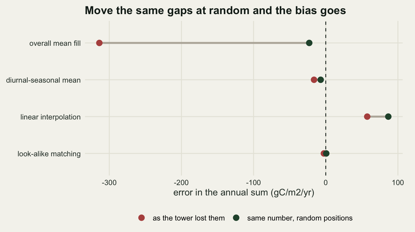
Everything so far has treated the 39.3 per cent missing as one quantity. It is not. The test is to keep the same number of missing half hours and change only where they fall: take the 3796 half hours removed by the friction velocity filter, put them back, and delete the same number of half hours chosen uniformly at random from the whole year instead. Downtime and weather stay exactly as they were.
set.seed(1212026)
n_us   <- sum(m_us)
m_rand <- rep(FALSE, n_tot)
m_rand[sample.int(n_tot, n_us)] <- TRUE
miss_b <- m_down | m_wx | m_rand
obs_b  <- !miss_b
gaps_b <- which(miss_b)

fb_mean <- nee_m; fb_mean[miss_b] <- mean(nee_m[obs_b])
fb_mdc  <- nee_m; fb_mdc[miss_b]  <- mdc_fill(nee_m, obs_b, gaps_b)
fb_lin  <- approx(which(obs_b), nee_m[obs_b], xout = seq_len(n_tot), rule = 2)$y
fb_mds  <- nee_m
fb_mds[miss_b] <- mds_fill(nee_m, obs_b, rg, ta, vpd, hod, gaps_b)$value

swap <- data.frame(
  method = sc$method,
  as_measured = sc$error,
  reshuffled = c(mean(nee_m[obs_b]) * n_tot * conv_gc - truth_annual,
                 sum(fb_mean) * conv_gc - truth_annual,
                 sum(fb_mdc) * conv_gc - truth_annual,
                 sum(fb_lin) * conv_gc - truth_annual,
                 sum(fb_mds) * conv_gc - truth_annual))
print(swap$method)
[1] "measured mean scaled up" "overall mean fill"
[3] "diurnal-seasonal mean" "linear interpolation"
[5] "look-alike matching" print(round(swap[, -1], 3)) as_measured reshuffled
1 -313.762 -22.895
2 -313.762 -22.895
3 -16.242 -7.036
4 57.473 86.677
5 -2.614 0.696print(round(c(gaps_original = mean(miss), gaps_reshuffled = mean(miss_b),
kept_mean_original = mean(nee_true[obs]),
kept_mean_reshuffled = mean(nee_true[obs_b]),
true_mean = mean(nee_true)), 4)) gaps_original gaps_reshuffled kept_mean_original
0.3930 0.3984 -1.7133
kept_mean_reshuffled true_mean
-0.9421 -0.8882 The reshuffled year is missing 39.84 per cent of its half hours against 39.3 per cent before, so if anything it has slightly less data. Mean imputation’s annual error goes from -313.76 gC/m2/yr to -22.89, a collapse of 92.7 per cent for no change in coverage whatever. The mean of the surviving half hours moves from -1.7133 umol/m2/s to -0.9421, against a true mean of -0.8882.
That is the finding the whole post exists for. Mean imputation of a year of flux is not biased because 39.3 per cent of the year is missing. It is biased because the missing half hours are the high-respiration ones. Delete just as many at random and the same crude method comes within 22.9 gC/m2/yr, and that residual is the downtime and weather mechanisms, which are mildly non-random themselves and are still worth 22.9 grams between them.
The better methods barely notice the swap. Look-alike matching goes from -2.61 to 0.7 gC/m2/yr and the diurnal-seasonal mean from -16.24 to -7.04 , because both of them condition on time of day and on the drivers, which is precisely the information that makes the friction velocity filter ignorable. Linear interpolation gets worse, 57.47 to 86.68, because scattering isolated gaps through the daytime asks it to draw chords across the steep parts of the diurnal cycle.
An honest error bar for the annual sum
The tower has to publish an uncertainty as well as a number. The usual first attempt propagates the random measurement error: each measured half hour carries a known error standard deviation, the errors are close to independent, so the standard error of their sum is the square root of the sum of their variances.
The honest version has to include the fact that a third of the year was invented. Repeating the whole exercise gives that: draw a fresh noise realisation, draw a fresh set of gaps from the same three mechanisms, fill with the look-alike matcher, and record the annual sum. The loop below runs two hundred replicates, which is modest but enough to pin a standard deviation to within about five per cent. It also runs a second version in which the noise is redrawn but the gap positions are held at the ones the tower actually suffered, so that the two sources can be told apart.
n_rep <- 200
ann_fixed <- numeric(n_rep)
ann_full  <- numeric(n_rep)
for (b in seq_len(n_rep)) {
  set.seed(500000 + b)
  yb <- nee_true + sig_v * (rexp(n_tot) - rexp(n_tot)) / sqrt(2)
  fa <- yb
  fa[miss] <- mds_fill(yb, obs, rg, ta, vpd, hod, gaps)$value
  ann_fixed[b] <- sum(fa) * conv_gc
  ub <- exp(-1.30 + 0.45 * wind_z + 0.55 * (rg / 900) -
              0.030 * pmax(ta, 0) * is_night + rnorm(n_tot, 0, 0.28))
  md_b <- rep(FALSE, n_tot)
  st_b <- sample.int(n_tot, n_out)
  ln_b <- 10 + rpois(n_out, 46)
  for (k in seq_len(n_out)) {
    md_b[st_b[k]:min(n_tot, st_b[k] + ln_b[k] - 1)] <- TRUE
  }
  md_b[long_idx] <- TRUE
  mm <- md_b | (runif(n_tot) < p_rain) | (runif(n_tot) < p_diag) |
    (is_night & ub < ustar_thr)
  fb <- yb
  fb[mm] <- mds_fill(yb, !mm, rg, ta, vpd, hod, which(mm))$value
  ann_full[b] <- sum(fb) * conv_gc
}

se_naive <- sqrt(sum(sig_v[obs]^2)) * conv_gc
qq <- quantile(ann_full, c(0.025, 0.975))
print(round(c(replicates = n_rep, truth = truth_annual,
              mean_annual = mean(ann_full), sd_annual = sd(ann_full),
              bias = mean(ann_full) - truth_annual,
              sd_fixed_gaps = sd(ann_fixed),
              naive_se = se_naive,
              ratio = sd(ann_full) / se_naive), 4))
replicates truth mean_annual sd_annual bias
200.0000 -338.9021 -339.6641 4.4053 -0.7620
sd_fixed_gaps naive_se ratio
4.5101 2.5893 1.7014 print(round(c(lower = unname(qq[1]), upper = unname(qq[2]),
width = unname(qq[2] - qq[1]),
diurnal_estimate = sc$annual[3],
diurnal_in_sd_units = (sc$annual[3] - mean(ann_full)) / sd(ann_full),
mean_fill_in_sd_units =
(sc$annual[2] - mean(ann_full)) / sd(ann_full)), 3)) lower upper width
-348.162 -331.135 17.026
diurnal_estimate diurnal_in_sd_units mean_fill_in_sd_units
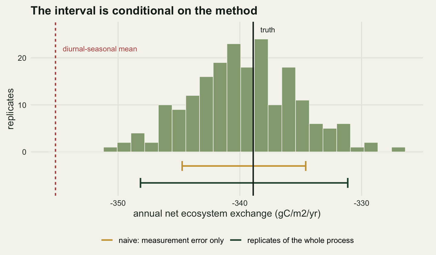
-355.145 -3.514 -71.051 The naive standard error is 2.589 gC/m2/yr. The spread of the annual sum over 200 replicates of the whole process is 4.405, larger by a factor of 1.701. A tower reporting the naive figure would publish an interval 41.2 per cent too narrow.
Where the extra comes from is not where I expected. Holding the gap positions fixed and redrawing only the noise gives 4.51 gC/m2/yr. Set that against the full spread quoted just above: a large part of the variation is already there with the gap positions frozen, so which half hours happen to be lost is not the main term. The gap between 2.589 and 4.405 is therefore not mainly a matter of gap placement. It is that a filled half hour inherits the noise of the handful of look-alikes it was averaged from, so the filled third of the year does not average its error down the way an independent measurement would, and the propagated measurement error leaves that out. In quadrature the filled half hours add 3.564 gC/m2/yr of their own.
The mean over replicates is -339.66 gC/m2/yr, and the figure to hold it against is the noise-free sum, -336.42, because every replicate draws its own noise while -338.9 carries the one draw the tower happened to get. On that comparison the matcher sits 3.24 gC/m2/yr low, about three quarters of the spread over the replicates, so it is not the unbiased filler the single year made it look. The 0.762 it appears to be out against the noisy year is that shift less the 2.48 grams of noise already sitting in the target. The central 95 per cent of the replicates runs from -348.16 to -331.14 gC/m2/yr, a width of 17.03, and it covers the noise-free sum without being centred on it.
Then the number that puts the interval in its place. The diurnal-seasonal mean, a method nobody would call unreasonable, returns -355.14 gC/m2/yr for this same year, which is 3.51 standard deviations from the centre of that interval and well outside it. Mean imputation is 71.1 standard deviations away. The uncertainty a gap-filling replicate study produces is conditional on the filling method, and the spread between methods is a term the interval does not contain and cannot. Hui et al (2004) made the same point from the other direction by treating gap filling as a multiple imputation problem, where the between-imputation variance is at least reported; Papale et al (2006), building the standard European processing chain, ended up quoting uncertainty from a set of processing choices rather than from one.
The honest limit
There is no truth column at a real tower, and that is not a detail. Every number above is a distance from a value the simulation set; in the field the only way to score a filling method is to hide half hours that were measured and put them back, which tests the method on the missingness it can already handle and says nothing about the half hours the friction velocity filter took. Moffat et al (2007) benchmarked on artificial gaps for exactly this reason, and were explicit that artificial gaps are a lower bound on the difficulty.
The simulation carries only random error. A real half-hourly flux has been through a coordinate rotation, a spectral correction for the frequency response of the instruments and a density correction for the effect of heat and water vapour transport on the measured mixing ratio, and each of those is a model with its own systematic error that does not cancel over a year. Energy balance closure at most sites falls short by ten to thirty per cent, a standing hint that something is being missed at the half-hourly level. Those errors sit on top of everything measured here and, unlike the noise, they do not average away.
The friction velocity filter is treated here as pure data loss, with a perfectly good value sitting behind the mask, and that is generous to it. The filter exists because the measured value on a calm night is itself wrong rather than merely unusual: carbon accumulates in the canopy air space instead of passing the sensor. The real situation is therefore worse than the simulated one, since the half hours removed are both non-randomly selected and unusable, and the fill has to reconstruct a quantity that was never measured well anywhere in that part of the driver space. Papale et al (2006) put the uncertainty from the threshold choice alone at a size comparable with everything else in the processing chain.
The drivers are complete here and they are not complete anywhere. When the mains fails it takes the radiation sensor with the analyser, so the look-alike matcher loses its matching variables precisely when it needs them, which is what the lower rungs of the ladder are for and why they fired 0.65 per cent of the time here instead of a realistic several per cent. That understates the difficulty of the long outage in particular. And the size of the bias reported above belongs to this site and this filter: a threshold of 0.2 m/s removing 42.6 per cent of night half hours is severe but not unusual, a windier site loses fewer and a sheltered valley more, and the annual error from mean imputation scales with that loss. What transfers is not the number -314 but the mechanism behind it.
Where to go next
The practical summary is short. Do not scale up a measured mean, because it is mean imputation and it inherits the full weight of whatever made the data missing. Condition the fill on time of day at minimum and on the drivers if they exist, since that is what converts a missing-not-at-random loss into one the fill can handle. Report the point-level error against the noise floor rather than on its own, because a root mean squared error only means something relative to what was achievable. And treat any single uncertainty figure as conditional: rerun the whole chain with a second filling method and quote the gap between them, since that gap is usually larger than the interval either method reports.
The threshold this post assumed is estimated in night-time flux and the u-star threshold, worth reading first if the filter’s severity is what you are unsure about. Once a filled series exists, splitting it into gross uptake and respiration is partitioning net flux into GPP and respiration, and the checks that decide whether the resulting budget can be published are in checking an annual flux budget. For the statistical side, multiple imputation by chained equations is the general machinery for turning a fill into an honest interval, and the flux literature’s version of it is Hui et al (2004); the reason it has not displaced the deterministic fill is partly inertia and partly that the between-imputation variance answers only one of the two questions asked here.
References
Falge E, Baldocchi D, Olson R, Anthoni P, Aubinet M, et al 2001 Agricultural and Forest Meteorology 107(1):43-69 (10.1016/S0168-1923(00)00225-2)
Reichstein M, Falge E, Baldocchi D, Papale D, Aubinet M, et al 2005 Global Change Biology 11(9):1424-1439 (10.1111/j.1365-2486.2005.001002.x)
Moffat AM, Papale D, Reichstein M, Hollinger DY, Richardson AD, et al 2007 Agricultural and Forest Meteorology 147(3-4):209-232 (10.1016/j.agrformet.2007.08.011)
Papale D, Reichstein M, Aubinet M, Canfora E, Bernhofer C, et al 2006 Biogeosciences 3(4):571-583 (10.5194/bg-3-571-2006)
Richardson AD, Hollinger DY, Burba G, Davis KJ, Flanagan LB, et al 2006 Agricultural and Forest Meteorology 136(1-2):1-18 (10.1016/j.agrformet.2006.01.007)
Richardson AD, Hollinger DY 2007 Agricultural and Forest Meteorology 147(3-4):199-208 (10.1016/j.agrformet.2007.06.004)
Hui D, Wan S, Su B, Katul G, Monson R, Luo Y 2004 Agricultural and Forest Meteorology 121(1-2):93-111 (10.1016/S0168-1923(03)00158-8)
Rubin DB 1976 Biometrika 63(3):581-592 (10.1093/biomet/63.3.581)
Lloyd J, Taylor JA 1994 Functional Ecology 8(3):315-323 (10.2307/2389824)