library(ggplot2)

te_pal <- list(forest = "#275139", green = "#2f8f63", sage = "#93a87f",
               clay = "#b5534e", gold = "#cda23f", line = "#dad9ca",
               ink = "#16241d", paper = "#f5f4ee")

theme_te <- function() {
  theme_minimal(base_size = 12) +
    theme(panel.grid.minor = element_blank(),
          panel.grid.major = element_line(colour = "#e7e6dc"),
          plot.background = element_rect(fill = "#f5f4ee", colour = NA),
          panel.background = element_rect(fill = "#f5f4ee", colour = NA),
          plot.title = element_text(face = "bold", colour = te_pal$ink),
          axis.title = element_text(colour = "#2c3a31"),
          axis.text = element_text(colour = "#2c3a31"))
}Filling cloud gaps in a satellite series
R
terra
remote sensing
missing data
ecology tutorial
Cloud gaps in a satellite NDVI series are not random: five fills scored in R against a known truth, and the ranking changes with the quantity you report.
A grazing study wants three numbers for every pixel of a ten kilometre square: how green the pixel was on average over the year, how far it swung between its winter floor and its summer peak, and which week it peaked. The input is a stack of eight-day NDVI composites at a resolution of two hundred and fifty metres, one year of them, forty-six layers. The window is forty by forty pixels, which is sixteen hundred pixels, small enough that everything below runs on a laptop in under a minute and small enough to hold several copies of the cube in memory while comparing them.
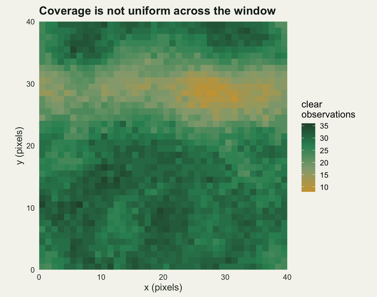
The stack has holes in it. Roughly two fifths of the pixel-dates are flagged cloudy and carry no value, and the holes are not sprinkled evenly: they arrive in slabs many pixels across, they concentrate in the wet months when the vegetation is doing everything interesting, and one band of the window is under orographic cloud so often that it ends the year with far fewer clear observations than the rest of the scene has. Whatever fills those holes decides all three of the numbers the study will report.
This post builds the cube with a known per-pixel truth, builds a cloud process with the three properties real cloud masks have plus the one that gets left out of tutorials, and scores five ways of dealing with the gaps against that truth on two things at once: the error at each filled observation, and the error in the three quantities anyone actually uses.
Three sibling posts carry the parts this one assumes. NDVI time series from a raster stack builds the cube and gets the layer dates and the per-pixel extraction right; harmonic regression on a seasonal raster fits the seasonal model that appears here as one of the five fills; checking a remote sensing covariate asks what happens when the finished layer becomes a predictor. A fourth, gap filling a flux time series, makes the same argument in a different medium, that the damage from missing data comes from the mechanism rather than the amount; this is the version with a spatial axis as well as a temporal one, and it measures that claim on its own cube rather than restating the flux results.
A cube that knows the answer
Two cover types share the window: a dry forest with a late, broad season and a grassland with an early, sharp one. The cover map is a smoothed random field cut at its median, so the two types form contiguous blocks rather than salt and pepper. On top of that sits a moisture gradient running west to east and a smooth per-pixel departure in level, amplitude and timing, so that neighbouring pixels resemble each other and distant ones do not. That last detail is the only reason a spatial fill has anything to work with. The seasonal shape is the asymmetric Gaussian used in phenology work, rising faster than it falls, because a curve a sinusoid can reproduce exactly would settle the harmonic comparison before it started.
library(terra)

n_side <- 40; n_pix <- n_side^2; n_lyr <- 46
doy <- seq(1, by = 8, length.out = n_lyr)
w_yr <- 2 * pi / 365.25
vec2mat <- function(v) matrix(v, n_side, n_side, byrow = TRUE)
mat2vec <- function(mm) as.vector(t(mm))

blur_op <- function(n, sd_pix) {
  dd <- outer(seq_len(n), seq_len(n),
              function(i, j) pmin(abs(i - j), n - abs(i - j)))
  kk <- exp(-0.5 * (dd / sd_pix)^2)
  kk / rowSums(kk)
}
sm_field <- function(bm) {
  n <- nrow(bm)
  z <- bm %*% matrix(rnorm(n * n), n, n) %*% t(bm)
  as.vector(scale(mat2vec(z)))
}

b_cover <- blur_op(n_side, 6); b_local <- blur_op(n_side, 4)
b_cloud <- blur_op(n_side, 3.2)
row_i <- rep(seq_len(n_side), each = n_side)
col_i <- rep(seq_len(n_side), times = n_side)

set.seed(20260803)
is_forest <- sm_field(b_cover) > 0
gradient <- 0.08 * (col_i - 1) / (n_side - 1)
base_v <- ifelse(is_forest, 0.34, 0.19) + gradient + 0.045 * sm_field(b_local)
amp_v <- ifelse(is_forest, 0.32, 0.50) + 0.055 * sm_field(b_local)
pk_v <- ifelse(is_forest, 200, 170) + 13 * sm_field(b_local)
wl_v <- ifelse(is_forest, 52, 42); wr_v <- ifelse(is_forest, 62, 52)
pl_v <- ifelse(is_forest, 3.0, 2.6); pr_v <- ifelse(is_forest, 2.2, 2.0)

asym_g <- function(dv, i) {
  z <- dv - pk_v[i]
  ifelse(z < 0, exp(-abs(z / wl_v[i])^pl_v[i]), exp(-abs(z / wr_v[i])^pr_v[i]))
}
ndvi_true <- outer(seq_len(n_pix), seq_len(n_lyr),
                   function(i, j) base_v[i] + amp_v[i] * asym_g(doy[j], i))
sd_obs <- 0.02
set.seed(51101)
noise <- matrix(rnorm(n_pix * n_lyr, 0, sd_obs), n_pix, n_lyr)
blank <- rast(nrows = n_side, ncols = n_side, xmin = 0, xmax = n_side,
              ymin = 0, ymax = n_side, nlyrs = n_lyr)
truth_cube <- setValues(blank, ndvi_true)
names(truth_cube) <- sprintf("d%03d", doy)

print(c(pixels = n_pix, layers = nlyr(truth_cube),
        forest_pixels = sum(is_forest), grass_pixels = sum(!is_forest),
        composite_length_days = 8))
pixels layers forest_pixels
1600 46 711
grass_pixels composite_length_days
889 8 print(round(c(ndvi_min = min(ndvi_true), ndvi_max = max(ndvi_true),
mean_amplitude_forest = mean(amp_v[is_forest]),
mean_amplitude_grass = mean(amp_v[!is_forest]),
mean_peak_forest = mean(pk_v[is_forest]),
mean_peak_grass = mean(pk_v[!is_forest]),
observation_noise_sd = sd_obs), 4)) ndvi_min ndvi_max mean_amplitude_forest
0.1370 0.8998 0.3085
mean_amplitude_grass mean_peak_forest mean_peak_grass
0.5092 199.8688 170.1050
observation_noise_sd
0.0200 The window holds 1600 pixels over 46 layers, 711 of them forest and 889 grassland. True NDVI runs from 0.137 to 0.9, the grassland swinging by 0.509 on average against the forest’s 0.308, and the two cover types peaking about 30 days apart. Every observation carries measurement noise with a standard deviation of 0.02, which is the floor: no filler can be scored below it on data it has actually seen.
The cube is held twice, as a SpatRaster for the spatial operations and mapping and as a 1600 by 46 matrix for the per-pixel work. Adding a bare numeric vector to a SpatRaster recycles it across layers rather than across cells and returns a cube with the wrong number of layers, so anything that is one number per cell is safer as a matrix, with setValues() used to put it back.
A cloud process with four properties
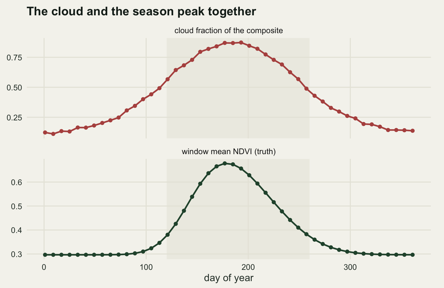
Real cloud masks do not remove independent pixels. Three properties of the missingness are documented well enough to be worth reproducing, and a fourth decides how honest the exercise is. The first is contiguity. Cloud arrives as blobs, so each date’s mask is generated by smoothing a field of white noise over a length scale of a few pixels and cutting it at the quantile that gives that date’s cloud fraction. The second is seasonal clustering. Wilson and Jetz (2016) built a global climatology of cloud frequency from two MODIS overpasses a day and found the seasonal cycle in cloud to be strong, spatially structured and closely tied to the vegetation cycle, which is exactly the awkward case: the cloudiest weeks are the green ones. The third is persistence. One band of the window, standing for a valley with orographic cloud, gets a fixed addition to its cloud field on every date, so its gaps are not spread evenly through the year and it never accumulates a full record.
The fourth property is contamination, the one that gets skipped. A cloud mask has two error rates, not one. Zhu and Woodcock (2012) report their Fmask algorithm at around ninety-six per cent overall accuracy for cloud on Landsat and are explicit that cloud shadow is the harder target; the later revision (Zhu and Woodcock 2014) improves the shadow and snow cases and still treats shadow omission as the residual problem. Omitted shadow and undetected thin cirrus leave no gap. They leave a number that looks like data and sits too low, so part of the retained record is corrupted rather than absent.
valley <- exp(-0.5 * ((row_i - 11) / 3.2)^2)
valley <- (valley - mean(valley)) / sd(valley)
persist_k <- 0.35; p_lo <- 0.08; p_hi <- 0.82
p_season <- p_lo + (p_hi - p_lo) * exp(-0.5 * ((doy - 185) / 58)^2)
p_cir <- 0.06; bias_shadow <- 0.085; bias_cirrus <- 0.035
det_shadow <- 0.7; det_cirrus <- 0.25

shift_tor <- function(v, dr, dc) {
  mm <- vec2mat(v)
  mat2vec(mm[((seq_len(n_side) - 1 - dr) %% n_side) + 1,
             ((seq_len(n_side) - 1 - dc) %% n_side) + 1])
}

make_cloud <- function(seed, pv) {
  set.seed(seed)
  cloud <- shadow <- cirrus <- matrix(FALSE, n_pix, n_lyr)
  for (j in seq_len(n_lyr)) {
    fld <- sm_field(b_cloud) + persist_k * valley
    thick <- fld > quantile(fld, 1 - pv[j], names = FALSE)
    thin <- fld > quantile(fld, max(0, 1 - pv[j] - p_cir), names = FALSE) & !thick
    shad <- as.logical(shift_tor(thick, 3, 2)) & !thick & !thin
    miss_sh <- shad & (runif(n_pix) > det_shadow)
    miss_ci <- thin & (runif(n_pix) > det_cirrus)
    cloud[, j] <- thick | (shad & !miss_sh) | (thin & !miss_ci)
    shadow[, j] <- miss_sh; cirrus[, j] <- miss_ci
  }
  list(cloud = cloud, shadow = shadow, cirrus = cirrus)
}

cmask <- make_cloud(4011, p_season)
contam <- bias_shadow * cmask$shadow + bias_cirrus * cmask$cirrus
y_obs <- ndvi_true + noise - contam
y_obs[cmask$cloud] <- NA
clear <- !cmask$cloud; gaps <- cmask$cloud; n_clear <- rowSums(clear)
wet <- doy >= 120 & doy <= 260; valley_pix <- valley > 1
frac_contam <- sum(clear & (cmask$shadow | cmask$cirrus)) / sum(clear)

print(round(c(overall_clear = mean(clear), overall_missing = mean(gaps),
              clear_in_growing_season = mean(clear[, wet]),
              clear_off_season = mean(clear[, !wet]),
              cloudiest_date_clear = min(colMeans(clear)),
              clearest_date_clear = max(colMeans(clear))), 4))
overall_clear overall_missing clear_in_growing_season
0.5660 0.4340 0.2648
clear_off_season cloudiest_date_clear clearest_date_clear
0.7596 0.1269 0.8888 print(round(c(clear_per_pixel_mean = mean(n_clear),
clear_per_pixel_sd = sd(n_clear),
fewest = min(n_clear), most = max(n_clear),
lower_decile = unname(quantile(n_clear, 0.1)),
valley_band_mean = mean(n_clear[valley_pix]),
elsewhere_mean = mean(n_clear[!valley_pix])), 3))clear_per_pixel_mean clear_per_pixel_sd fewest
26.036 5.562 8.000
most lower_decile valley_band_mean
36.000 17.000 16.846
elsewhere_mean
27.985 print(round(c(contaminated_share_of_retained = frac_contam,
omitted_shadow_share = sum(clear & cmask$shadow) / sum(clear),
thin_cirrus_share = sum(clear & cmask$cirrus) / sum(clear),
mean_pull_when_contaminated = mean(contam[clear & contam > 0]),
rmse_of_retained_values = sqrt(mean((y_obs[clear] -
ndvi_true[clear])^2)),
noise_floor = sd_obs), 4))contaminated_share_of_retained omitted_shadow_share
0.1145 0.0353
thin_cirrus_share mean_pull_when_contaminated
0.0792 0.0504
rmse_of_retained_values noise_floor
0.0274 0.0200 The seasonal profile runs from 0.08 cloudy at the dry end of the year to 0.82 at midsummer, and the two contamination biases pull a retained value down by 0.085 for omitted shadow and 0.035 for thin cirrus, with 30 per cent of shadows and 75 per cent of thin cirrus escaping the mask.
The window keeps 56.6 per cent of its pixel-dates, which is an ordinary figure for a cloudy region, and that single number hides everything. In the growing season only 26.48 per cent survive against 75.96 per cent off season, and the worst date keeps 12.69 per cent of the window while the best keeps 88.88 per cent. Per pixel the count of clear observations runs from 8 to 36 out of 46, with a standard deviation of 5.56; the valley band averages 16.8 clear observations against 28 for the rest of the window.
Of the observations that survive the mask, 11.45 per cent are contaminated: 3.53 per cent omitted shadow and 7.92 per cent undetected thin cirrus, pulled down by 0.0504 on average. The consequence is in the last two numbers: the retained values have a root mean squared error of 0.0274 against a truth they are supposed to record exactly up to the 0.02 measurement noise. Before any filling happens, the clear-sky data are already 1.37 times worse than the instrument.
Blob geometry decides whether a spatial fill can work at all, and the statistic that captures it is how often a cloudy pixel’s immediate neighbours are cloudy too.
nb_share <- vapply(seq_len(n_lyr), function(j) {
  cl <- gaps[, j]
  nb <- (shift_tor(cl, 1, 0) + shift_tor(cl, -1, 0) +
           shift_tor(cl, 0, 1) + shift_tor(cl, 0, -1)) / 4
  mean(nb[cl])
}, 0)
print(round(c(neighbour_also_cloudy = mean(nb_share),
              marginal_cloud_fraction = mean(gaps),
              ratio = mean(nb_share) / mean(gaps)), 4))
neighbour_also_cloudy marginal_cloud_fraction ratio
0.8437 0.4340 1.9440 A pixel picked at random is cloudy 43.4 per cent of the time; a pixel next to a cloudy one is cloudy 84.37 per cent of the time, a factor of 1.94. Gaps come in slabs, and inside a slab a spatial fill is extrapolating rather than interpolating, with no way to say so.
Which mechanism is which
Rubin (1976) split missingness into three cases by what the probability of a value being absent depends on, and the split is worth applying here one mechanism at a time, because the four properties above land in different boxes. Missing data: MCAR, MAR and MNAR works through the taxonomy on a rectangular dataset; the point of repeating the exercise on a cube is that a single scene can carry all three at once.
truth_mean <- rowMeans(ndvi_true)
date_truth <- colMeans(ndvi_true)
print(round(c(truth_mean_over_all_cells = mean(ndvi_true),
              truth_mean_over_clear_cells = mean(ndvi_true[clear]),
              selection_shift = mean(ndvi_true[clear]) - mean(ndvi_true),
              cor_date_cloudiness_with_date_ndvi =
                cor(1 - colMeans(clear), date_truth),
              cor_pixel_clear_count_with_pixel_ndvi = cor(n_clear, truth_mean),
              truth_when_contaminated = mean(ndvi_true[clear & contam > 0]),
              truth_when_uncontaminated = mean(ndvi_true[clear & contam == 0])),
            4))
truth_mean_over_all_cells truth_mean_over_clear_cells
0.3985 0.3330
selection_shift cor_date_cloudiness_with_date_ndvi
-0.0655 0.9438
cor_pixel_clear_count_with_pixel_ndvi truth_when_contaminated
-0.3909 0.3935
truth_when_uncontaminated
0.3252 Blob placement within a date is missing completely at random with respect to NDVI. The cloud field is generated independently of the surface, so which pixel a blob happens to cover on a given date says nothing about that pixel’s greenness. It costs precision and nothing else.
Seasonal clustering is missing at random. The correlation between a date’s cloud fraction and that date’s mean true NDVI is 0.944, so the missingness depends strongly on the value. It depends on it only through the date, and the date is recorded for every layer, so conditioning on the date makes the missingness ignorable. The taxonomy then predicts the consequence: an estimator that conditions on date is safe and a marginal average over whatever survived is not. The mean of the truth over the clear cells is 0.333 against 0.3985 over all of them, a shift of -0.0655 NDVI units that exists before any analysis is done.
Persistent pixels are also missing at random, this time on pixel identity rather than date. The correlation between a pixel’s clear count and its annual mean truth is -0.391 here. The valley band is not a random subsample of the window. Because pixel identity is recorded, a per-pixel analysis is unaffected, but any scene-level average that pools pixels without weighting inherits the difference between that band and the rest.
Contamination is outside the taxonomy altogether, which is why it is easy to forget. Rubin’s three cases classify which values are absent, and a contaminated observation is present. Forced into the taxonomy by treating the mask’s failure as the missingness event, it is missing not at random: whether a shadow is masked depends on how dark the pixel is, and that darkness is exactly what corrupts the value. The awkward part is in the last two numbers: the true NDVI at contaminated cells averages 0.3935 against 0.3252 at clean ones, because shadow and cirrus occur next to cloud and cloud occurs in the green season. The contamination lands disproportionately on the observations that were already scarce.
Five ways to deal with the gaps
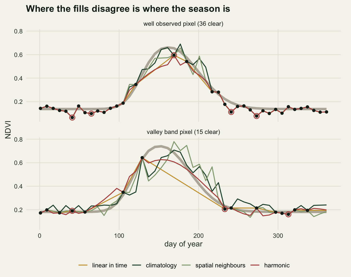
The fills are the ones a working analysis reaches for. The first is not a fill at all: drop the gaps and compute each pixel’s summaries from whatever it has. The second is per-pixel linear interpolation in time. The third is a climatology, the mean of every clear pixel of the same cover type on the same date, which is the seasonal profile a pixel of that type is expected to follow. The fourth is spatial, the mean of the pixel’s clear neighbours on the same date from a five by five window, widening to eleven by eleven where the smaller window has nothing and falling back to the date’s clear-scene mean where even that fails. The fifth is a harmonic reconstruction, two harmonics fitted to the pixel’s own clear dates and predicted onto the missing ones, the method of Roerink, Menenti and Verhoef (2000) in its plainest form, without their iterative outlier rejection. Five coefficients fitted to a handful of observations is an extrapolation with nothing behind it, so a pixel that never reaches three clear observations per coefficient takes the climatology instead.
obs_cube <- setValues(blank, y_obs)
f5 <- values(focal(obs_cube, w = 5, fun = "mean", na.rm = TRUE))
f11 <- values(focal(obs_cube, w = 11, fun = "mean", na.rm = TRUE))

spatial_fill <- function(yy, clr, w5, w11) {
  out <- yy
  date_mean <- colMeans(yy, na.rm = TRUE)
  for (j in seq_len(n_lyr)) {
    gj <- !clr[, j]; fill <- w5[, j]
    fill[is.na(fill)] <- w11[is.na(fill), j]
    fill[is.na(fill)] <- date_mean[j]
    out[gj, j] <- fill[gj]
  }
  out
}
clim_fill <- function(yy, clr) {
  out <- yy
  for (j in seq_len(n_lyr)) {
    v <- yy[, j]; m <- clr[, j]
    fill <- ifelse(is_forest, mean(v[m & is_forest]), mean(v[m & !is_forest]))
    out[!m, j] <- fill[!m]
  }
  out
}
lin_fill <- function(yy, clr) {
  out <- yy
  for (i in seq_len(n_pix)) {
    m <- clr[i, ]
    out[i, !m] <- approx(doy[m], yy[i, m], xout = doy[!m], rule = 2)$y
  }
  out
}
x_harm <- cbind(1, cos(w_yr * doy), sin(w_yr * doy),
                cos(2 * w_yr * doy), sin(2 * w_yr * doy))
k_min <- 15
harm_fill <- function(yy, clr, backup) {
  out <- yy; n_back <- 0
  for (i in seq_len(n_pix)) {
    m <- clr[i, ]
    if (sum(m) >= k_min) {
      cf <- qr.solve(x_harm[m, , drop = FALSE], yy[i, m])
      out[i, !m] <- (x_harm[!m, , drop = FALSE] %*% cf)[, 1]
    } else {
      out[i, !m] <- backup[i, !m]
      n_back <- n_back + 1
    }
  }
  list(value = out, n_back = n_back)
}

cube_clim <- clim_fill(y_obs, clear)
cube_spat <- spatial_fill(y_obs, clear, f5, f11)
cube_lin <- lin_fill(y_obs, clear)
harm_out <- harm_fill(y_obs, clear, cube_clim)
cube_harm <- harm_out$value; n_no5 <- sum(is.na(f5) & gaps)

print(c(gaps = sum(gaps), gaps_with_no_clear_neighbour_in_5x5 = n_no5,
        harmonic_coefficients = ncol(x_harm),
        minimum_clear_for_a_harmonic_fit = k_min,
        pixels_falling_back_to_climatology = harm_out$n_back))
gaps gaps_with_no_clear_neighbour_in_5x5
31943 14649
harmonic_coefficients minimum_clear_for_a_harmonic_fit
5 15
pixels_falling_back_to_climatology
67 The spatial fill has no clear pixel inside its five by five window for 14649 of the 31943 gaps, which is 45.86 per cent of them, and 67 pixels never reach 15 clear observations and take the climatology instead. Both numbers are properties of the cloud process rather than of the code, and both are invisible in the finished cube.
Two scorecards that disagree
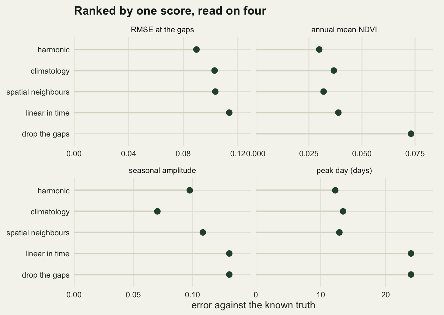
Every filled cube is scored twice. The first score is the root mean squared error at the gaps only, against the noise-free truth, which is the number a gap-filling paper reports. The second is the error in the three quantities the grazing study will actually publish: each pixel’s annual mean NDVI, its seasonal amplitude taken as the largest value of the year minus the smallest, and the day of year on which it peaked, compared on the circle so that January and December are close together.
truth_amp <- apply(ndvi_true, 1, max) - apply(ndvi_true, 1, min)
truth_peak <- doy[apply(ndvi_true, 1, which.max)]
circ_gap <- function(a, b) { d <- abs(a - b) %% 365; pmin(d, 365 - d) }

tally <- function(nm, rm, am, ap, pk) data.frame(
  method = nm, rmse = rm,
  mean_err = mean(am - truth_mean), mean_rmse = sqrt(mean((am - truth_mean)^2)),
  amp_err = mean(ap - truth_amp), amp_rmse = sqrt(mean((ap - truth_amp)^2)),
  peak_mae = mean(circ_gap(pk, truth_peak)))

score_cube <- function(cube, nm, gp)
  tally(nm, sqrt(mean((cube[gp] - ndvi_true[gp])^2)), rowMeans(cube),
        apply(cube, 1, max) - apply(cube, 1, min),
        doy[apply(cube, 1, which.max)])

score_drop <- function(yy, clr, nm)
  tally(nm, NA_real_, rowSums(ifelse(clr, yy, 0)) / rowSums(clr),
        vapply(seq_len(n_pix), function(i) diff(range(yy[i, clr[i, ]])), 0),
        vapply(seq_len(n_pix),
               function(i) doy[clr[i, ]][which.max(yy[i, clr[i, ]])], 0))

m_lab <- c("drop the gaps", "linear in time", "climatology",
           "spatial neighbours", "harmonic")
sc <- rbind(score_drop(y_obs, clear, m_lab[1]),
            score_cube(cube_lin, m_lab[2], gaps),
            score_cube(cube_clim, m_lab[3], gaps),
            score_cube(cube_spat, m_lab[4], gaps),
            score_cube(cube_harm, m_lab[5], gaps))
rk <- function(v) rank(ifelse(is.na(v), Inf, v), ties.method = "min")
sc$r_rmse <- rk(sc$rmse); sc$r_mean <- rk(sc$mean_rmse)
sc$r_amp <- rk(sc$amp_rmse); sc$r_peak <- rk(sc$peak_mae)
print(sc$method)
[1] "drop the gaps" "linear in time" "climatology"
[4] "spatial neighbours" "harmonic" print(round(sc[, 2:7], 4)) rmse mean_err mean_rmse amp_err amp_rmse peak_mae
1 NA -0.0685 0.0731 -0.0409 0.1310 23.895
2 0.1137 -0.0275 0.0389 -0.0409 0.1310 23.895
3 0.1029 -0.0204 0.0368 0.0401 0.0703 13.430
4 0.1034 -0.0231 0.0319 0.0877 0.1087 12.865
5 0.0896 -0.0188 0.0299 -0.0150 0.0976 12.230print(sc[, c("r_rmse", "r_mean", "r_amp", "r_peak")]) r_rmse r_mean r_amp r_peak
1 5 5 4 4
2 4 4 4 4
3 2 3 1 3
4 3 2 3 2
5 1 1 2 1gv <- function(nm, col) sc[[col]][match(nm, sc$method)]The gap-level scorecard is unsurprising. The harmonic wins it at 0.0896, the climatology and the spatial fill are level at 0.1029 and 0.1034, and linear interpolation trails at 0.1137. Anyone stopping here would call the harmonic best by 12.9 per cent and the climatology and the spatial fill interchangeable, since they differ by 0.49 per cent.
The seasonal amplitude reverses part of that. The climatology fill has an amplitude error of 0.0703 against the harmonic’s 0.0976, so the method that won the gap-level score loses the amplitude by 38.83 per cent, and the two methods the gap-level score could not separate differ by 54.53 per cent on it. Amplitude is a range statistic, so it responds to the spread of the filled values rather than to their average accuracy. The spatial fill scatters neighbour values around roughly the right level and inflates the range by 0.0877 on average; the harmonic smooths and shrinks it by 0.015; the climatology, which inserts a curve of about the right shape, inflates it by 0.0401 and keeps the smallest amplitude RMSE of the five.
The sharpest version of the point sits in the two rows nobody would compare. Dropping the gaps and interpolating linearly between them give amplitude errors of 0.131 and 0.131, and peak-day errors of 23.895 and 23.895 days. Those are not similar numbers; they are the same numbers, to every digit computed. Linear interpolation with rule = 2 never returns a value outside the range of the observations it is given, so it cannot restore a peak that was never seen, and the position of the maximum it does produce is the position of the observed maximum. It halves the annual-mean error, from 0.0731 to 0.0389, and buys exactly nothing on the other two quantities. A method can be a genuine improvement on one target and a null operation on another.
Where the cloud falls, not how much of it
To show that the seasonal clustering is doing the damage, keep the amount of cloud and change only its placement. The same generator runs again with a flat seasonal profile at the mean of the real one, so the wet months are no longer singled out. Everything else is identical: the same seed, the same blobs, the same valley, the same contamination rules.
p_flat <- rep(mean(p_season), n_lyr)
cmask_u <- make_cloud(4011, p_flat)
y_u <- ndvi_true + noise - bias_shadow * cmask_u$shadow -
  bias_cirrus * cmask_u$cirrus
y_u[cmask_u$cloud] <- NA
clear_u <- !cmask_u$cloud; gaps_u <- cmask_u$cloud
obs_cube_u <- setValues(blank, y_u)
f5u <- values(focal(obs_cube_u, w = 5, fun = "mean", na.rm = TRUE))
f11u <- values(focal(obs_cube_u, w = 11, fun = "mean", na.rm = TRUE))
cl_u <- clim_fill(y_u, clear_u)
sc_u <- rbind(score_drop(y_u, clear_u, m_lab[1]),
              score_cube(lin_fill(y_u, clear_u), m_lab[2], gaps_u),
              score_cube(cl_u, m_lab[3], gaps_u),
              score_cube(spatial_fill(y_u, clear_u, f5u, f11u), m_lab[4], gaps_u),
              score_cube(harm_fill(y_u, clear_u, cl_u)$value, m_lab[5], gaps_u))

swap <- data.frame(method = m_lab, clustered = sc$mean_err,
                   uniform = sc_u$mean_err, clustered_rmse = sc$mean_rmse,
                   uniform_rmse = sc_u$mean_rmse)
swap$removed_pct <- 100 * (1 - abs(swap$uniform / swap$clustered))
print(round(c(clustered_missing = mean(gaps), uniform_missing = mean(gaps_u),
              clustered_gaps = sum(gaps), uniform_gaps = sum(gaps_u),
              extra_gaps_in_uniform = sum(gaps_u) - sum(gaps)), 4))
clustered_missing uniform_missing clustered_gaps
0.4340 0.4518 31943.0000
uniform_gaps extra_gaps_in_uniform
33254.0000 1311.0000 print(swap$method)[1] "drop the gaps" "linear in time" "climatology"
[4] "spatial neighbours" "harmonic" print(round(swap[, -1], 4)) clustered uniform clustered_rmse uniform_rmse removed_pct
1 -0.0685 -0.0121 0.0731 0.0284 82.3013
2 -0.0275 -0.0092 0.0389 0.0176 66.5392
3 -0.0204 -0.0162 0.0368 0.0359 20.7491
4 -0.0231 -0.0207 0.0319 0.0312 10.2694
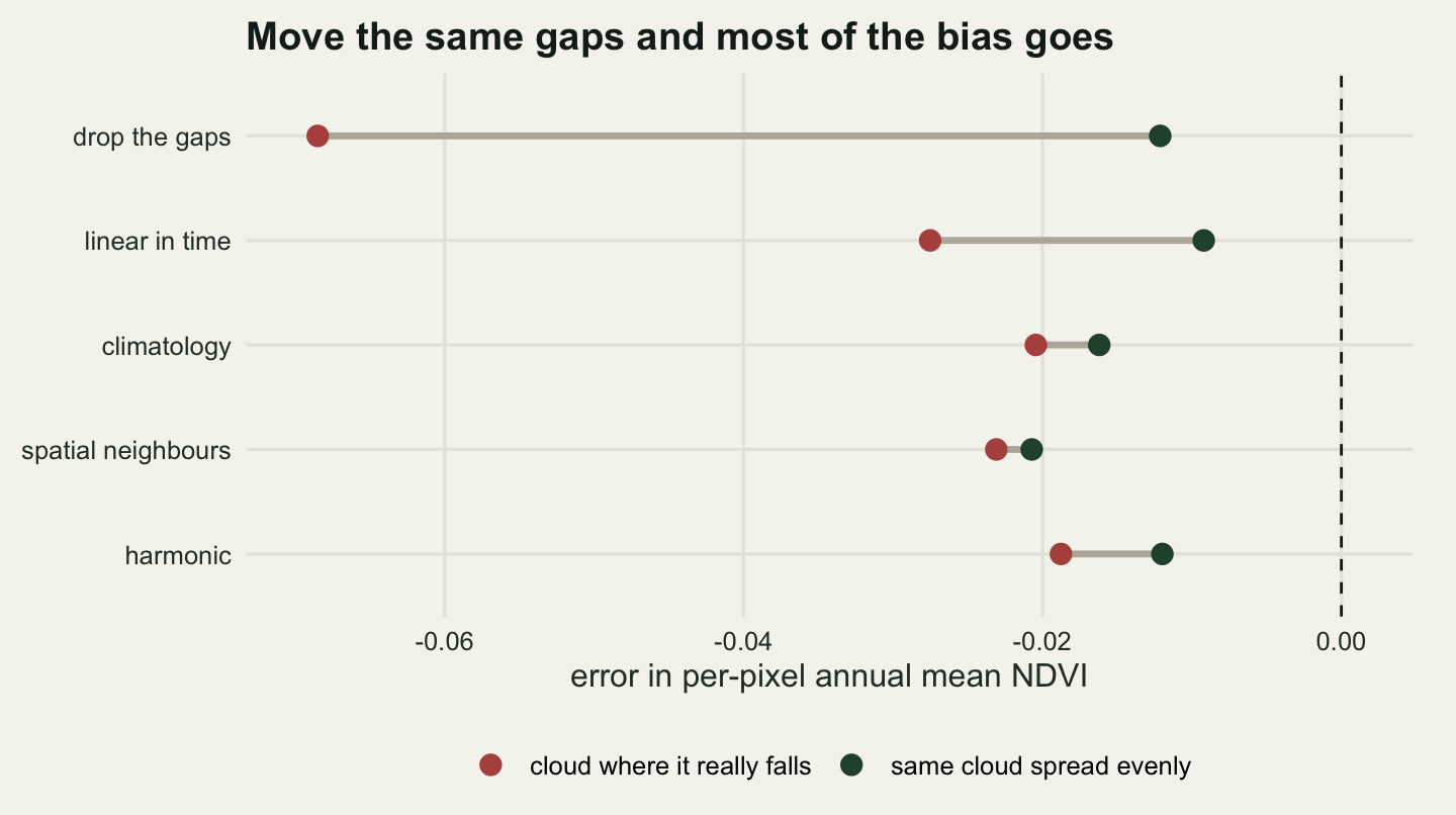
5 -0.0188 -0.0120 0.0299 0.0255 36.1669gu <- function(nm, col) swap[[col]][match(nm, swap$method)]The reshuffled year is missing 45.18 per cent of its pixel-dates against 43.4 per cent before, so it has 1311 more gaps rather than fewer. The complete-case annual mean, the estimator a hurried analysis uses, has an error of -0.0685 NDVI units with the cloud in its real seasonal place and -0.0121 with the same cloud spread evenly: 82.3 per cent of the bias disappears when the placement changes and nothing else does. Linear interpolation loses 66.54 per cent of its bias the same way.
The methods that condition on date barely notice. The climatology goes from -0.0204 to -0.0162, the spatial fill from -0.0231 to -0.0207. Both of them estimate the missing value from other pixels observed on the same date, which is precisely the conditioning that makes a MAR mechanism ignorable, so removing the clustering takes almost nothing away from them because they were not paying for it.
Does the amount matter, once the shape of the profile is fixed? The sweep scales the whole cloud profile up and down and pairs each level with a uniform counterpart at matched coverage.
amount <- c(0.5, 0.75, 1, 1.25)
sweep_tab <- do.call(rbind, lapply(amount, function(fa) {
  pv <- pmin(0.95, fa * p_season)
  one <- function(cx) {
    yy <- ndvi_true + noise - bias_shadow * cx$shadow - bias_cirrus * cx$cirrus
    yy[cx$cloud] <- NA
    clr <- !cx$cloud
    am <- rowSums(ifelse(clr, yy, 0)) / rowSums(clr)
    c(miss = mean(cx$cloud), err = mean(am - truth_mean))
  }
  a <- one(make_cloud(4011, pv))
  b <- one(make_cloud(4011, rep(mean(pv), n_lyr)))
  data.frame(scale_factor = fa, missing_clustered = a["miss"],
             err_clustered = a["err"], missing_uniform = b["miss"],
             err_uniform = b["err"])
}))
rownames(sweep_tab) <- NULL
sweep_tab$ratio <- sweep_tab$err_clustered / sweep_tab$err_uniform
print(round(sweep_tab, 4))
scale_factor missing_clustered err_clustered missing_uniform err_uniform
1 0.50 0.2384 -0.0334 0.2469 -0.0068
2 0.75 0.3406 -0.0504 0.3506 -0.0087
3 1.00 0.4340 -0.0685 0.4518 -0.0121
4 1.25 0.5133 -0.0856 0.5422 -0.0155
ratio
1 4.9271
2 5.7781
3 5.6501
4 5.5290worst_uniform <- sweep_tab$err_uniform[4]
mildest_clustered <- sweep_tab$err_clustered[1]This did not come out the way the setup suggested it would. The bias does not stop caring about the amount of cloud once the clustering is fixed: it scales almost linearly with it, from -0.0334 at 23.8 per cent missing to -0.0856 at 51.3 per cent. What is stable is the ratio. At each of the four coverage levels the clustered placement produces between 4.93 and 5.78 times the bias of a uniform placement with the same coverage, so clustering acts as a multiplier on the damage rather than as its source.
That multiplier is large enough to swamp the amount. Uniform cloud at 54.2 per cent missing, the worst coverage tested, gives an annual-mean error of -0.0155. Clustered cloud at 23.8 per cent missing, less than half as much data lost, gives -0.0334, which is 2.16 times worse. Doubling the cloud in a scene is a smaller problem than moving it into the growing season, and the coverage percentage that gets quoted in a methods section carries none of that.
The contamination nobody masks
No filler can address the third mechanism, because to a filler a contaminated observation is data. Running the comparison again with the biases switched off, leaving the mask exactly as it was, separates the two.
y_cln <- ndvi_true + noise
y_cln[gaps] <- NA
obs_cube_c <- setValues(blank, y_cln)
f5c <- values(focal(obs_cube_c, w = 5, fun = "mean", na.rm = TRUE))
f11c <- values(focal(obs_cube_c, w = 11, fun = "mean", na.rm = TRUE))
cl_c <- clim_fill(y_cln, clear)
sc_c <- rbind(score_drop(y_cln, clear, m_lab[1]),
              score_cube(lin_fill(y_cln, clear), m_lab[2], gaps),
              score_cube(cl_c, m_lab[3], gaps),
              score_cube(spatial_fill(y_cln, clear, f5c, f11c), m_lab[4], gaps),
              score_cube(harm_fill(y_cln, clear, cl_c)$value, m_lab[5], gaps))
cont_tab <- data.frame(method = m_lab, with_contamination = sc$mean_err,
                       without = sc_c$mean_err, rmse_with = sc$rmse,
                       rmse_without = sc_c$rmse)
cont_tab$share_pct <- 100 * (1 - cont_tab$without / cont_tab$with_contamination)
print(cont_tab$method)
[1] "drop the gaps" "linear in time" "climatology"
[4] "spatial neighbours" "harmonic" print(round(cont_tab[, -1], 4)) with_contamination without rmse_with rmse_without share_pct
1 -0.0685 -0.0625 NA NA 8.8137
2 -0.0275 -0.0195 0.1137 0.1065 29.1254
3 -0.0204 -0.0115 0.1029 0.0978 43.5205
4 -0.0231 -0.0077 0.1034 0.0930 66.8589
5 -0.0188 -0.0107 0.0896 0.0829 43.1640direct_pull <- mean(clear) * mean(contam[clear])
full_bias <- mean(rowMeans(ndvi_true + noise - contam) - truth_mean)
best_gain <- cont_tab$with_contamination[4] - cont_tab$without[4]
carried <- best_gain + direct_pull
print(round(c(bias_if_nothing_were_masked = full_bias,
direct_pull_on_retained_cells = -direct_pull,
contamination_cost_to_spatial_fill = best_gain,
amplification_factor = best_gain / full_bias,
carried_into_the_gaps = carried), 5)) bias_if_nothing_were_masked direct_pull_on_retained_cells
-0.00311 -0.00327
contamination_cost_to_spatial_fill amplification_factor
-0.01544 4.96596
carried_into_the_gaps
-0.01217 cont_get <- function(nm, col) cont_tab[[col]][match(nm, cont_tab$method)]Contamination is 11.45 per cent of the retained observations and it accounts for far more than that share of the error. For the spatial fill the annual-mean bias falls from -0.0231 to -0.0077 when the biases are switched off, so 66.86 per cent of what is left after a good fill is contamination rather than missingness. The harmonic loses 43.16 per cent of its bias the same way and the climatology 43.52 per cent, while the complete-case estimator, whose error is dominated by the seasonal selection, loses only 8.81 per cent. The pattern runs one way only: the crude estimators are dominated by the seasonal selection, and once a fill has removed that, contamination is a large share of what is left across the three fills that condition on date.
The last block explains why the effect is so much bigger than the contamination itself. If nothing at all were masked and only the shadow and cirrus biases were applied, the annual mean of the cube would be off by -0.00311, since contaminated cells are a small minority of a complete year. Under the real mask the same contamination costs the spatial fill -0.0154, an amplification of 4.97 times. Of that, -0.00327 is the direct pull on the retained cells and the remaining -0.0122 is the fill carrying the contamination forward into the gaps. A shadow that escapes the mask is not one bad pixel: it is one bad pixel plus every gap that was filled from it.
Nothing in the finished cube marks these cells. They pass the mask, they lie inside the plausible range, and a smoother of the kind Chen et al (2004) apply to NDVI series, which treats points below a locally fitted curve as suspect, would read a run of shadow-depressed values in the wettest fortnight as the signal it is meant to preserve. Hird and McDermid (2009) compared six such noise-reduction filters on real series and found the choice among them to matter less than what the series had already been through.
A quality layer, and what it tracks
The count of clear observations per pixel is free, already in the mask, and the one honest description of how far the filled cube can be trusted from place to place.
best_err <- rowMeans(cube_spat) - truth_mean
harm_err <- rowMeans(cube_harm) - truth_mean
peak_err_sp <- circ_gap(doy[apply(cube_spat, 1, which.max)], truth_peak)
peak_err_hm <- circ_gap(doy[apply(cube_harm, 1, which.max)], truth_peak)
fifth <- cut(n_clear, breaks = quantile(n_clear, seq(0, 1, 0.2)),
             include.lowest = TRUE, labels = FALSE)
qtab <- data.frame(
  fifth = 1:5,
  clear_mean = tapply(n_clear, fifth, mean),
  abs_err_spatial = tapply(abs(best_err), fifth, mean),
  abs_err_harmonic = tapply(abs(harm_err), fifth, mean),
  peak_err_spatial = tapply(peak_err_sp, fifth, mean),
  peak_err_harmonic = tapply(peak_err_hm, fifth, mean))
print(round(qtab, 4))
fifth clear_mean abs_err_spatial abs_err_harmonic peak_err_spatial
1 1 16.9403 0.0436 0.0360 13.4448
2 2 24.3731 0.0259 0.0247 12.9664
3 3 28.1546 0.0187 0.0156 13.0023
4 4 30.5016 0.0151 0.0122 11.9369
5 5 32.5825 0.0142 0.0100 12.9072
peak_err_harmonic
1 13.1582
2 13.2355
3 12.7026
4 10.9274
5 10.0206print(round(c(pearson_spatial = cor(n_clear, abs(best_err)),
pearson_harmonic = cor(n_clear, abs(harm_err)),
spearman_spatial = cor(n_clear, abs(best_err),
method = "spearman"),
worst_fifth_over_best =
qtab$abs_err_spatial[1] / qtab$abs_err_spatial[5]), 4)) pearson_spatial pearson_harmonic spearman_spatial
-0.5210 -0.4578 -0.4485
worst_fifth_over_best
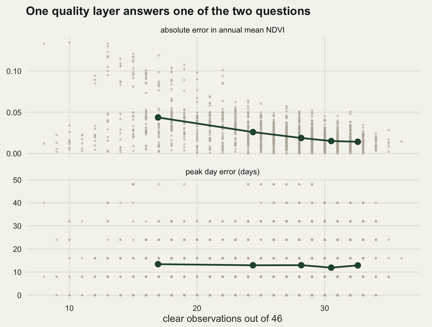
3.0802 q_cor <- cor(n_clear, abs(best_err))The correlation between a pixel’s clear count and the absolute error in its annual mean is -0.521 for the spatial fill and -0.458 for the harmonic. Across quintiles of coverage the spatial fill’s mean absolute error runs from 0.0436 in the worst-covered fifth, which averages 16.9 clear observations, to 0.0142 in the best, at 32.6 observations: a factor of 3.08 across one scene, in a cube whose every cell now carries a number and looks equally finished.
The same layer can be read against the peak day as well. The spatial fill’s peak-day error goes from 13.44 days in the worst-covered fifth to 12.91 days in the best, a ratio of 1.04. The way the fill is built matters here. The spatial fill takes every gap from the pixel’s neighbours on the same date, or from the date’s clear-scene mean where even the wider window is empty, so the crest of a filled series is set by the scene around the pixel as much as by the pixel’s own record, and the pixel’s own clear count is not the only thing that sets it. The harmonic, which fits the pixel’s own clear dates, gives 13.16 days in the worst fifth against 10.02 in the best, a gap of 31.31 per cent, next to the annual mean’s factor of 3.08.
That is the case for carrying the layer rather than a single coverage figure. Clear count tracks the annual-mean error, and a per-pixel count of clear observations inside the growing season costs one more line of code to carry next to it.
The honest limit
The truth column here is a simulation and the cloud process is invented. Its three structural properties are not: contiguity, seasonal clustering and persistent pixels are all documented, the seasonal one at global scale by Wilson and Jetz (2016). The numbers that come out of the comparison, though, are numbers about this generator. A scene with shorter blob correlation lengths, a flatter cloud season or a smoother surface would reorder the fills, and Kandasamy et al (2013), comparing eight smoothing and gap-filling methods on MODIS leaf area index across a range of biomes, found that pattern: no method dominating everywhere, the ranking shifting with the site. The transferable part is the shape of the argument, not the league table.
Real masks also fail in the other direction. Everything above treats the mask as too permissive. Masks are also too aggressive over bright surfaces: fresh snow, dry sand and bright bare soil are the classic commission errors, which is why the second Fmask paper (Zhu and Woodcock 2014) spends its effort on separating snow from cloud. A commission error deletes a genuine clear observation, and it does so in a spatially and seasonally structured way, adding another MAR mechanism keyed to surface brightness rather than to weather. Nothing here measures that.
The most important limit is what a filled cube is. Every value at a gap is a model output, and the model that produced it has uncertainty that the cube does not record. Anything computed from the filled cube as if it were data will report an interval that is too narrow: the point made in general terms in single imputation: bias and variance, where an unbiased single fill still undercovers because a single completed dataset cannot express the doubt about the fill itself. Here the gaps are 43.4 per cent of the cube, so a regression of an ecological response on filled NDVI is fitting to a predictor that is more than two fifths model output, and the standard error it prints will not know that. Weiss et al (2014), gap filling remotely sensed series at continental scale, made the same point from the operational side, that the filled product has to be delivered with a description of how it was filled and where.
Where to go next
Three things follow. The cheapest is the quality layer: keep the clear count, which tracks the annual-mean error, keep a growing-season clear count next to it, and carry both into whatever the cube feeds. The second is to choose the fill by the quantity being reported rather than by the score the gap-filling literature quotes, since the two disagreed here by enough to change the answer. The third is to treat the mask as a two-sided instrument with its own error rates.
The harmonic fill used here is the plainest version, one fit per pixel with no outlier rejection and no borrowing of strength from neighbours. Harmonic regression on a seasonal raster sets the method up properly; the natural extension, which this post does not attempt, is to fit the harmonic to the pixel and its neighbours jointly, so that a valley pixel with a short record borrows its shape from the hillside above it and keeps only its own level.
References
Rubin DB 1976 Biometrika 63(3):581-592 (10.1093/biomet/63.3.581)
Roerink GJ, Menenti M, Verhoef W 2000 International Journal of Remote Sensing 21(9):1911-1917 (10.1080/014311600209814)
Chen J, Jonsson P, Tamura M, Gu Z, Matsushita B, Eklundh L 2004 Remote Sensing of Environment 91(3-4):332-344 (10.1016/j.rse.2004.03.014)
Hird JN, McDermid GJ 2009 Remote Sensing of Environment 113(1):248-258 (10.1016/j.rse.2008.09.003)
Zhu Z, Woodcock CE 2012 Remote Sensing of Environment 118:83-94 (10.1016/j.rse.2011.10.028)
Kandasamy S, Baret F, Verger A, Neveux P, Weiss M 2013 Biogeosciences 10(6):4055-4071 (10.5194/bg-10-4055-2013)
Zhu Z, Woodcock CE 2014 Remote Sensing of Environment 152:217-234 (10.1016/j.rse.2014.06.012)
Weiss DJ, Atkinson PM, Bhatt S, Mappin B, Hay SI, Gething PW 2014 ISPRS Journal of Photogrammetry and Remote Sensing 98:106-118 (10.1016/j.isprsjprs.2014.10.001)
Wilson AM, Jetz W 2016 PLoS Biology 14(3):e1002415 (10.1371/journal.pbio.1002415)