library(ggplot2)

te_pal <- list(forest = "#275139", green = "#2f8f63", sage = "#93a87f",
               clay = "#b5534e", gold = "#cda23f", line = "#dad9ca",
               ink = "#16241d", paper = "#f5f4ee")

theme_te <- function() {
  theme_minimal(base_size = 12) +
    theme(panel.grid.minor = element_blank(),
          panel.grid.major = element_line(colour = "#e7e6dc"),
          plot.background = element_rect(fill = "#f5f4ee", colour = NA),
          panel.background = element_rect(fill = "#f5f4ee", colour = NA),
          plot.title = element_text(face = "bold", colour = te_pal$ink),
          axis.title = element_text(colour = "#2c3a31"),
          axis.text = element_text(colour = "#2c3a31"))
}Harmonic regression on a seasonal raster
R
remote sensing
time series
terra
ecology tutorial
Fit a sine and cosine pair per pixel to a year of NDVI composites in R, map amplitude and peak day, and measure what the raw seasonal maximum gets wrong.
A window 1200 metres on a side over a lowland mosaic: rough grassland on free-draining gravels in the south, a block of oak and hornbeam in the north, and a ragged band of encroaching scrub between them. The satellite archive holds one year of 8-day NDVI composites over that window, 46 layers, on a 30 metre grid, so the cube is 40 pixels by 40 pixels with 46 observations at each. It is a deliberately small window: everything below runs on a laptop in under a minute.
The question is not what the NDVI was on any particular date. It is what the seasonal cycle looks like at each pixel: how far the vegetation swings between its winter floor and its summer ceiling, and when it peaks. Those two numbers, an amplitude and a phase, are what goes into the habitat model or the comparison between management compartments, and they have to be recovered from 46 noisy values per pixel, with clouds deleting some of them and the composites eight days apart to begin with. The obvious way to get the peak is to ask which layer is largest, which is one line of code and what most people write first. It is also the estimator this post is mainly about, because a fitted seasonal curve beats it by a factor of four in these data.
NDVI time series from a raster stack built a cube of this shape and took per-pixel summaries off it: means, maxima, an integral over the season. This post fits a model to the time axis instead, which is a different object, because a summary throws away the shape and a model parametrises it. Raster data in R with terra covers single-layer work and is not repeated. Filling cloud gaps in a satellite series is about reconstructing missing observations; the section on missing dates below asks only what an unfilled gap does to a fitted coefficient. Checking a remote sensing covariate takes the outputs of this post and asks whether they deserve to be in a model at all. Two older posts set the other boundaries. Phenological trends and temperature estimates timing from ground observation: somebody walked the transect and wrote down a date, and here the same quantity is read off a reflectance curve by a machine that never visited the site. And circular data and the von Mises distribution owns the arithmetic of angles, which matters because a phase is an angle and forgetting that is one of the standard mistakes in this workflow.
Six things get measured: how well amplitude, phase and mean are recovered when the truth is known; how the answer moves as harmonics are added; how far the raw seasonal maximum is from the truth compared with two fitted alternatives; what an unevenly missing set of dates does; which direction a season-shaped gap pushes the amplitude; and how large the per-pixel standard error on the amplitude is before anybody carries it into another model.
A cube with a known answer inside it
Simulated data, because the point is to measure error and that needs a truth. Each pixel gets a mean NDVI, an amplitude, a peak day and a small second harmonic, all varying smoothly across the window through a woodland index running from open grass in the south to closed canopy in the north. The second harmonic is what makes the curve asymmetric, and a single cosine cannot express asymmetry at all. These parameters lean it towards a slow rise and a quicker fall, which is the other way round from a real deciduous canopy: a property of the simulated truth, not a claim about phenology. For measuring error what matters is that the curve leans at all.
suppressPackageStartupMessages(library(terra))

n_side <- 40
n_cell <- n_side^2
n_lyr <- 46
doy <- seq(1, 361, by = 8)
omega <- 2 * pi / 365

tmpl <- rast(nrows = n_side, ncols = n_side, xmin = 0, xmax = 1200,
             ymin = 0, ymax = 1200, crs = "EPSG:32634")
xy_cell <- crds(tmpl)
g_east <- xy_cell[, 1] / 1200; g_north <- xy_cell[, 2] / 1200
wood <- plogis(7 * (g_north - 0.5 + 0.28 * sin(3.1 * g_east)))
mean_true <- 0.34 + 0.16 * wood
amp_true <- 0.13 + 0.17 * wood + 0.02 * g_east
peak_par <- 150 + 36 * wood + 10 * g_north
amp2_true <- 0.008 + 0.022 * wood

day_fine <- 1:365
ang_fine <- omega * (matrix(day_fine, n_cell, 365, byrow = TRUE) - peak_par)
sig_fine <- mean_true + amp_true * cos(ang_fine) + amp2_true * sin(2 * ang_fine)
peak_true <- day_fine[max.col(sig_fine, ties.method = "first")]

ang_obs <- omega * (matrix(doy, n_cell, n_lyr, byrow = TRUE) - peak_par)
sig_obs <- mean_true + amp_true * cos(ang_obs) + amp2_true * sin(2 * ang_obs)

sd_noise <- 0.04
set.seed(20260803)
obs_mat <- sig_obs + matrix(rnorm(n_cell * n_lyr, 0, sd_noise), n_cell, n_lyr)

ndvi <- setValues(rast(tmpl, nlyr = n_lyr), obs_mat)
names(ndvi) <- sprintf("d%03d", doy)

print(c(pixels = ncell(ndvi), layers = nlyr(ndvi),
        composite_days = doy[2] - doy[1], first_doy = doy[1],
        last_doy = doy[n_lyr]))
pixels layers composite_days first_doy last_doy
1600 46 8 1 361 print(round(c(mean_lo = min(mean_true), mean_hi = max(mean_true),
amp_lo = min(amp_true), amp_hi = max(amp_true),
peak_lo = min(peak_true), peak_hi = max(peak_true),
noise_sd = sd_noise), 4)) mean_lo mean_hi amp_lo amp_hi peak_lo peak_hi noise_sd
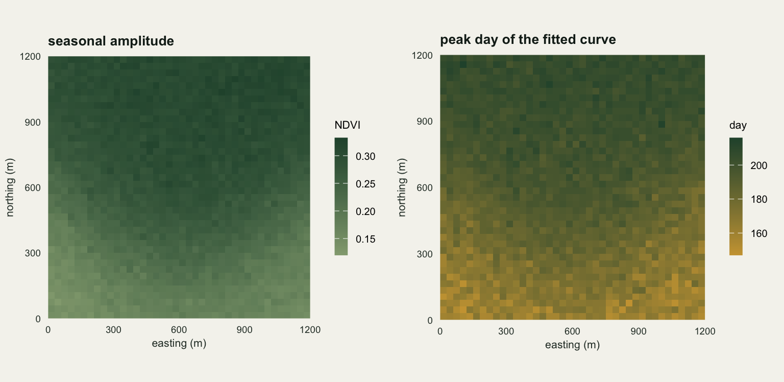
0.3455 0.4993 0.1361 0.3153 158.0000 206.0000 0.0400 The cube holds 1600 pixels and 46 layers, one composite every 8 days from day 1 to day 361. True amplitude runs from 0.136 in the driest grass to 0.315 in the closed canopy, and the true peak day, defined as the argmax of the noiseless annual curve, runs from day 158 to day 206. Per-observation noise has a standard deviation of 0.04, which is an ordinary figure for a composited vegetation index once residual cloud, aerosol and view-angle effects are in it.
One terra habit is worth stating first, because it fails silently. A SpatRaster plus a bare numeric vector recycles across layers, not across cells, so adding a 1600-element per-pixel vector to a 46-layer cube produces a cube with hundreds of layers and no error. The safe route is the one used above: build the values as a matrix of cells by layers, hand it to setValues(), check nlyr().
One pixel, one linear model
Write \(y_t\) for the NDVI of a pixel at day of year \(t\) and \(\omega = 2\pi/365\). The one-harmonic model is
\[y_t = \mu + a\cos(\omega t) + b\sin(\omega t) + \varepsilon_t\]
which looks like a curve-fitting problem and is not one. The pair \(\cos(\omega t)\) and \(\sin(\omega t)\) are known numbers once the dates are known, so \(\mu\), \(a\) and \(b\) enter linearly and the whole thing is lm(). No optimiser, no starting values, no convergence to worry about. That is why harmonic regression is the workhorse in this corner of remote sensing. Jakubauskas, Legates and Kastens (2002) used the amplitudes and phases of the first few harmonics of an AVHRR NDVI series as classification features, the direct ancestor of using them as ecological covariates; Zhu and Woodcock (2014) put the same form at the centre of continuous change detection, fitting it to a stable period and flagging a pixel when new observations fall outside the prediction interval, which only works because refitting everywhere is cheap; and Verbesselt, Hyndman, Newnham and Culvenor (2010) take the complementary route in BFAST, separating a seasonal component from a piecewise trend and testing for breaks in each.
The two coefficients are then rewritten as an amplitude and a phase, because that is what anybody wants to look at:
\[a\cos(\omega t) + b\sin(\omega t) = A\cos(\omega t - \phi), \qquad A = \sqrt{a^2 + b^2}, \qquad \phi = \operatorname{atan2}(b, a)\]
and the phase converts to a day of year as \(\phi/\omega\), taken modulo 365. Adding more harmonics means adding \(\cos(2\omega t)\), \(\sin(2\omega t)\) and so on: still linear, still lm().
harm_design <- function(days, n_harm) {
  des <- matrix(1, length(days), 1 + 2 * n_harm)
  colnames(des) <- c("mean", as.vector(rbind(paste0("cos", seq_len(n_harm)),
                                             paste0("sin", seq_len(n_harm)))))
  for (j in seq_len(n_harm)) {
    des[, 2 * j] <- cos(2 * pi * j * days / 365)
    des[, 2 * j + 1] <- sin(2 * pi * j * days / 365)
  }
  des
}

pix_id <- cellFromXY(tmpl, cbind(315, 915))
pix_dat <- data.frame(ndvi = obs_mat[pix_id, ], cos1 = cos(omega * doy),
                      sin1 = sin(omega * doy))
fit_pix <- lm(ndvi ~ cos1 + sin1, data = pix_dat)
print(round(summary(fit_pix)$coefficients, 5))
Estimate Std. Error t value Pr(>|t|)
(Intercept) 0.49198 0.00618 79.61077 0
cos1 -0.28323 0.00870 -32.54016 0
sin1 -0.05196 0.00877 -5.92202 0cf_pix <- coef(fit_pix)
amp_pix <- sqrt(cf_pix[2]^2 + cf_pix[3]^2)
phase_pix <- (atan2(cf_pix[3], cf_pix[2]) / omega) %% 365
lmfit_pix <- lm.fit(harm_design(doy, 1), obs_mat[pix_id, ])$coefficients
print(round(c(intercept = unname(cf_pix[1]), true_mean = mean_true[pix_id],
amplitude = unname(amp_pix), true_amplitude = amp_true[pix_id],
phase_day = unname(phase_pix), true_peak_day = peak_true[pix_id],
woodland_index = wood[pix_id]), 4)) intercept true_mean amplitude true_amplitude phase_day
0.4920 0.4941 0.2880 0.2990 193.0409
true_peak_day woodland_index
203.0000 0.9631 print(round(c(max_gap_lm_vs_lmfit = max(abs(cf_pix - lmfit_pix))), 12))max_gap_lm_vs_lmfit
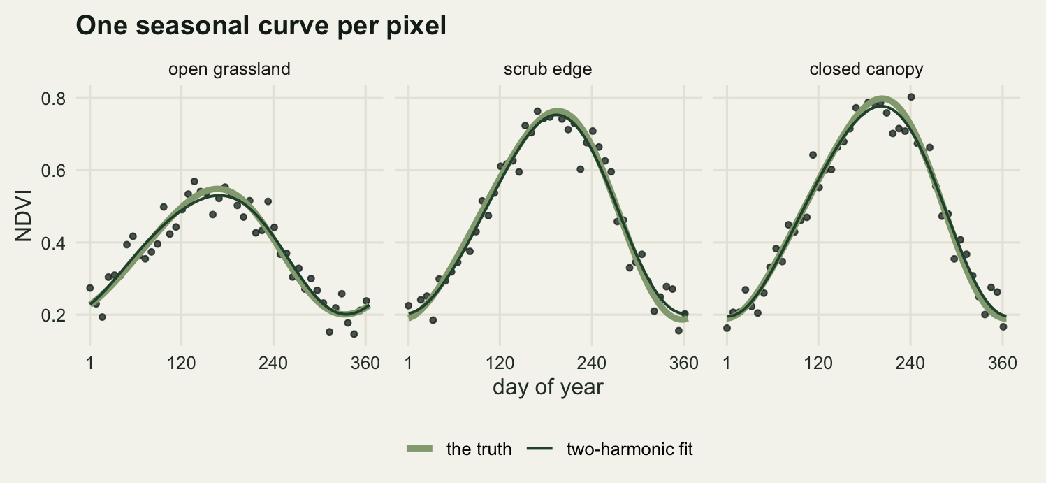
0 At this pixel the intercept comes out at 0.492 against a true mean of 0.4941, and the amplitude at 0.288 against a true 0.299. The phase converts to day 193 while the true peak of the pixel’s curve is day 203, a gap of 10 days that is not noise and will be taken apart later. lm() and lm.fit() on the same design return identical coefficients, which matters only because the per-pixel loop below uses the second one for speed.
The phase is an angle, and angles do not average
Once a phase has been converted to a day of year it looks like an ordinary number, and the moment somebody averages peak days over a management unit or differences them between years, the branch cut bites. Day 362 and day 3 are six days apart, not 359.
wrap_days <- c(356, 362, 3, 9, 14)
naive_mean <- mean(wrap_days)
wrap_ang <- omega * wrap_days
vec_mean <- (atan2(mean(sin(wrap_ang)), mean(cos(wrap_ang))) / omega) %% 365
resultant <- sqrt(mean(cos(wrap_ang))^2 + mean(sin(wrap_ang))^2)

print(round(c(arithmetic_mean_day = naive_mean, vector_mean_day = vec_mean,
              resultant_length = resultant, error_days = naive_mean - vec_mean), 3))
arithmetic_mean_day vector_mean_day resultant_length error_days
148.800 2.802 0.990 145.998 Five pixels whose peaks straddle the new year have an arithmetic mean peak day of 148.8, which is in late May. The vector mean, taken by averaging the unit vectors and converting back with atan2(), is day 2.8, and it is the right answer: the arithmetic version is off by 146 days. The resultant length 0.99 measures the agreement, near one when the phases coincide and near zero when they cancel. Fisher (1993) is the standard treatment and the base R mechanics are in the circular post. Nothing in this window peaks near the new year, so the problem never surfaces here, but it is exactly what a semi-arid system with a winter growing season does, and it fails silently when it does.
Fitting every pixel with app()
terra::app() applies a function to the vector of layer values at each cell, which is exactly the shape a per-pixel time series has. The function returns a vector of coefficients, so the result is a multi-layer raster with one layer per coefficient. Two harmonics gives five: a mean and two cosine and sine pairs.
des2 <- harm_design(doy, 2)
harm_r <- app(ndvi, function(v) lm.fit(des2, v)$coefficients)
names(harm_r) <- colnames(des2)
print(harm_r)
class : SpatRaster
size : 40, 40, 5 (nrow, ncol, nlyr)
resolution : 30, 30 (x, y)
extent : 0, 1200, 0, 1200 (xmin, xmax, ymin, ymax)
coord. ref. : WGS 84 / UTM zone 34N (EPSG:32634)
source(s) : memory
names : mean, cos1, sin1, cos2, sin2
min values : 0.330629, -0.327367, -0.083869, -0.037725, -0.018976
max values : 0.516825, -0.104717, 0.09443, 0.033952, 0.052607cf2 <- values(harm_r)
cf_direct <- t(qr.coef(qr(des2), t(obs_mat)))
print(c(coef_layers = nlyr(harm_r),
agrees_with_matrix_solve = max(abs(cf2 - cf_direct)) < 1e-12)) coef_layers agrees_with_matrix_solve
5 1 The output carries 5 layers and reproduces a single matrix solve of the same design exactly, which is worth checking once and then relying on: the sweeps later in the post use the matrix form, because running app() inside a replicate loop would spend its time on raster overheads for no gain.
fine2 <- harm_design(day_fine, 2)
circ_gap <- function(a, b) ((a - b + 182.5) %% 365) - 182.5

amp_hat <- sqrt(cf2[, "cos1"]^2 + cf2[, "sin1"]^2)
phase_hat <- (atan2(cf2[, "sin1"], cf2[, "cos1"]) / omega) %% 365
peak_hat <- day_fine[max.col(cf2 %*% t(fine2), ties.method = "first")]

amp_r <- setValues(rast(tmpl), amp_hat)
peak_r <- setValues(rast(tmpl), peak_hat)
print(c(amp_layers = nlyr(amp_r), peak_layers = nlyr(peak_r)))
amp_layers peak_layers
1 1 amp_err <- amp_hat - amp_true
peak_err <- circ_gap(peak_hat, peak_true)
mean_err <- cf2[, "mean"] - mean_true
amp_mae <- median(abs(amp_err))
amp_p90 <- unname(quantile(abs(amp_err), 0.9))
peak_mae <- median(abs(peak_err))
peak_p90 <- unname(quantile(abs(peak_err), 0.9))
print(round(c(mean_median_abs_err = median(abs(mean_err)),
amp_median_abs_err = amp_mae, amp_p90_abs_err = amp_p90,
amp_median_pct_err = 100 * median(abs(amp_err / amp_true)),
amp_bias = mean(amp_err)), 5))mean_median_abs_err amp_median_abs_err amp_p90_abs_err amp_median_pct_err
0.00391 0.00555 0.01370 2.20723
amp_bias
-0.00033 print(round(c(peak_median_abs_err_days = peak_mae, peak_p90_days = peak_p90,
peak_bias_days = mean(peak_err),
peak_worst_days = max(abs(peak_err))), 3))peak_median_abs_err_days peak_p90_days peak_bias_days
3.000 7.000 -0.072
peak_worst_days
17.000 Against a known truth the two-harmonic fit recovers the annual mean to a median absolute error of 0.0039 NDVI units and the amplitude to 0.0056, or 2.21 per cent of the amplitude being estimated, with a ninetieth percentile of 0.0137: a tail about two and a half times the median rather than an order of magnitude away. Peak day comes back with a median absolute error of 3 days, a ninetieth percentile of 7 days and a mean signed error of -0.07 days, the worst pixel being 17 days out.
How many harmonics
One harmonic is a symmetric hump. Two can lean. Three can carry a shoulder. The usual way to choose is a fit statistic, so start there and then ask whether the fit statistic is answering the question.
fit_harm <- function(n_harm, keep = seq_len(n_lyr), y_mat = obs_mat) {
  des <- harm_design(doy[keep], n_harm)
  yk <- y_mat[, keep, drop = FALSE]
  cf <- t(qr.coef(qr(des), t(yk)))
  rss <- rowSums((yk - cf %*% t(des))^2)
  list(cf = cf, des = des, rss = rss, npar = ncol(des),
       amp = sqrt(cf[, 2]^2 + cf[, 3]^2),
       peak = day_fine[max.col(cf %*% t(harm_design(day_fine, n_harm)),
                               ties.method = "first")],
       rse = sqrt(rss / (length(keep) - ncol(des))),
       r2 = 1 - rss / rowSums((yk - rowMeans(yk))^2))
}

k_grid <- 1:3
scan_out <- lapply(k_grid, fit_harm)
k_tab <- data.frame(
  harmonics = k_grid,
  parameters = sapply(scan_out, function(s) s$npar),
  resid_sd = sapply(scan_out, function(s) median(s$rse)),
  r_squared = sapply(scan_out, function(s) median(s$r2)),
  amp_mae = sapply(scan_out, function(s) median(abs(s$amp - amp_true))),
  amp_bias = sapply(scan_out, function(s) mean(s$amp - amp_true)),
  peak_mae = sapply(scan_out, function(s) mean(abs(circ_gap(s$peak, peak_true)))),
  peak_bias = sapply(scan_out, function(s) mean(circ_gap(s$peak, peak_true))))
print(round(k_tab, 5))
harmonics parameters resid_sd r_squared amp_mae amp_bias peak_mae peak_bias
1 1 3 0.04305 0.95088 0.00555 -0.00031 9.54750 -9.54500
2 2 5 0.03963 0.96196 0.00555 -0.00033 3.31063 -0.07187
3 3 7 0.03959 0.96401 0.00556 -0.00034 5.60500 -0.14875bic_mat <- sapply(scan_out, function(s)
n_lyr * log(s$rss / n_lyr) + (s$npar + 1) * log(n_lyr))
aic_mat <- sapply(scan_out, function(s)
n_lyr * log(s$rss / n_lyr) + 2 * (s$npar + 1))
bic_pick <- tabulate(max.col(-bic_mat, ties.method = "first"), 3)
aic_pick <- tabulate(max.col(-aic_mat, ties.method = "first"), 3)
print(rbind(harmonics = k_grid, bic_pixels = bic_pick, aic_pixels = aic_pick)) [,1] [,2] [,3]
harmonics 1 2 3
bic_pixels 670 886 44
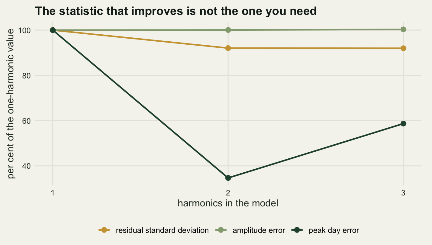
aic_pixels 320 988 292The fit statistics behave the way fit statistics always do. Median residual standard deviation falls from 0.0430 at one harmonic to 0.0396 at two and 0.0396 at three, and the median R squared climbs from 0.9509 through 0.9620 to 0.9640: read that column alone and three harmonics looks harmless. The columns that matter say something else. Mean absolute error in the estimated peak day is 9.55 days at one harmonic, drops to 3.31 days at two, and rises again to 5.6 days at three: the third harmonic makes the estimate 69.3 per cent worse while making the residuals look better. What the third harmonic is fitting is the noise, and the argmax of a curve is a sharp functional of that curve, so a wiggle worth 0.00003 NDVI units of residual moves the crest by days.
The amplitude, by contrast, does not care. Median absolute error is 0.00555, 0.00555 and 0.00556 at one, two and three harmonics, and the bias is under 0.00034 throughout. That is not luck. On a complete year of evenly spaced dates the harmonic columns are mutually orthogonal, so leaving out the second harmonic cannot contaminate the first, and adding a third costs almost nothing in variance. Hold on to that sentence: the next section but one takes the even spacing away and the property goes with it.
Per-pixel information criteria do not settle it either. BIC picks one harmonic at 670 pixels, two at 886 and three at 44; AIC, being more permissive, picks three at 292 pixels, or 18.2 per cent of the window. Selecting per pixel would hand a third harmonic to hundreds of pixels that measurably do not want one, and produce a peak-day map whose estimator changes from place to place.
Two harmonics, fitted everywhere, is the recommendation these numbers support, and it is conditional on the shape of this signal: one growing season a year with a moderately asymmetric crest. A genuine double season, a spring flush and an autumn flush, needs at least the second harmonic to represent the two peaks and probably a third to place them, and a canopy that sits on a plateau for four months needs more terms than either. The way to find out is the comparison run above, against a truth or against withheld dates, not the R squared column.
Three ways to read the peak day, and the gap between them
Here is the comparison the post exists for. Three estimators of the same quantity, the day of year on which a pixel’s greenness crests:
- the argmax of the raw series, that is the day of the composite with the largest NDVI;
- the argmax of the fitted two-harmonic curve, evaluated on a daily grid;
- the analytic phase of the first harmonic, \(\phi/\omega\).
The first is the line most people write. The third is what you get if you read the phase coefficient off the model and call it the peak, which is common and is not the same as the second whenever the curve is asymmetric.
raw_peak <- doy[max.col(obs_mat, ties.method = "first")]
clean_peak <- doy[max.col(sig_obs, ties.method = "first")]

est_days <- list("raw seasonal maximum" = raw_peak,
                 "argmax of the fitted curve" = peak_hat,
                 "phase of the first harmonic" = phase_hat)
peak_tab <- do.call(rbind, lapply(names(est_days), function(nm) {
  e <- circ_gap(est_days[[nm]], peak_true)
  data.frame(estimator = nm, mean_abs_days = mean(abs(e)),
             median_abs_days = median(abs(e)), bias_days = mean(e),
             sd_days = sd(e), p90_abs_days = unname(quantile(abs(e), 0.9)),
             worse_8d = mean(abs(e) > 8))
}))
print(round(peak_tab[, -1], 4))
mean_abs_days median_abs_days bias_days sd_days p90_abs_days worse_8d
1 13.6763 12.0000 -0.1188 17.0193 28.0000 0.6250
2 3.3106 3.0000 -0.0719 4.3187 7.0000 0.0562
3 9.5459 9.7902 -9.5435 2.3897 12.3119 0.7825print(peak_tab$estimator)[1] "raw seasonal maximum" "argmax of the fitted curve"
[3] "phase of the first harmonic"raw_floor <- mean(abs(circ_gap(clean_peak, peak_true)))
gain_ratio <- peak_tab$mean_abs_days[1] / peak_tab$mean_abs_days[2]
print(round(c(noiseless_raw_argmax_error = raw_floor,
quantisation_floor = (doy[2] - doy[1]) / 4,
raw_over_fitted = gain_ratio, raw_sd_days = peak_tab$sd_days[1],
fitted_sd_days = peak_tab$sd_days[2]), 4))noiseless_raw_argmax_error quantisation_floor
2.1437 2.0000
raw_over_fitted raw_sd_days
4.1310 17.0193
fitted_sd_days
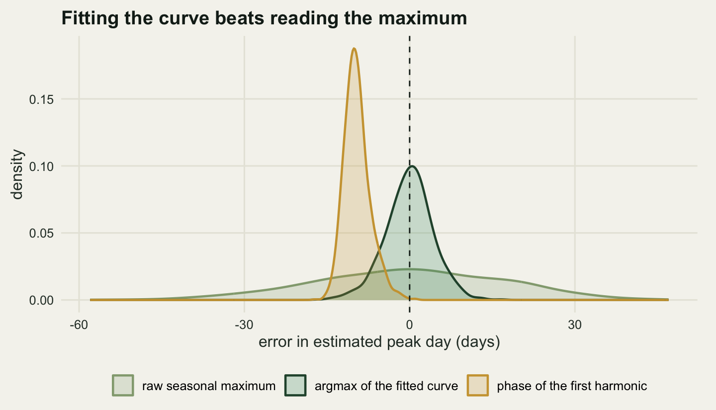
4.3187 The raw seasonal maximum is off by 13.68 days on average, with a ninetieth percentile of 28 days and 62.5 per cent of pixels more than a composite interval from the truth. The fitted curve’s argmax averages 3.31 days, a factor of 4.13 better, from exactly the same 46 numbers.
Two separate things hurt the raw estimator, and the numbers separate them. Run the same argmax on the noiseless signal and the error is still 2.14 days, because an 8-day product can only return one of 46 dates and the average distance from a uniformly placed true peak to the nearest of them is 2 days. That is the compositing floor, and no care with the raw series gets under it. Noise then takes the raw estimator from 2.14 days to 13.68, because the top of a seasonal curve is nearly flat: over the three composites either side of the crest the signal changes by less than the observation noise, so which is largest is close to a coin toss. The fitted curve has neither problem. It is evaluated on a daily grid, so no compositing floor applies, and all 46 observations contribute to where the crest is put rather than just the winner.
The third estimator is the interesting failure, and it is the most precise of the three. Its standard deviation is 2.39 days against 4.32 for the fitted argmax, because it uses two coefficients rather than four and is a smooth function of them instead of a maximum. It is also biased by -9.54 days and puts 78.2 per cent of pixels more than a composite interval from the truth. The bias is less a defect than a statement that it estimates a different quantity: the phase of the first harmonic is the crest of the symmetric part of the curve, and when the second harmonic leans the curve towards a slow green-up the crest moves later while the phase stays put. Here the lean is worth 9.5 days, a fifth of the whole grassland-to-woodland difference the map is meant to show.
The rule out of this section: fit the model, then find the maximum of the fitted curve numerically. Do not read the peak off the phase coefficient unless the curve is known to be symmetric, and do not take the argmax of the raw composites at all. Harmonic fitting is in any case not the usual route to a phenological date: Zhang and colleagues (2003) fit piecewise logistic functions and take the extremes of the rate of change of curvature as the transitions, which suits a fast green-up better than a low order Fourier series does.
When the dates go missing
Everything above assumed 46 evenly spaced composites. Real archives do not deliver that. Cloud, snow, sensor outages and quality flags remove observations, and they do not remove them at random across the year: in a temperate summer it is convective cloud, in a monsoon system it is a solid three months of nothing. Roerink, Menenti and Verhoef (2000) built HANTS around this problem, wrapping the same regression in an iterative rejection loop that discards observations lying below the fitted curve, on the grounds that cloud almost always depresses a vegetation index, and then predicting the missing dates from the fit. That reconstruction is the gap-filling post’s subject; the question here is narrower. Three scenarios, all dropping the same number of dates so that sample size is held fixed and only the pattern changes: nine at random, nine consecutive composites lost across the spring green-up, and nine consecutive composites lost across the senescence, each run over 50 noise replicates.
spring_out <- which(doy >= 97 & doy <= 161)
autumn_out <- which(doy >= 193 & doy <= 257)
keep_full <- seq_len(n_lyr)
keep_spring <- setdiff(keep_full, spring_out)
keep_autumn <- setdiff(keep_full, autumn_out)
n_drop <- length(spring_out)
print(c(dropped_per_scenario = n_drop, retained = n_lyr - n_drop,
        spring_gap_from = doy[min(spring_out)], spring_gap_to = doy[max(spring_out)],
        autumn_gap_from = doy[min(autumn_out)], autumn_gap_to = doy[max(autumn_out)]))
dropped_per_scenario retained spring_gap_from
9 37 97
spring_gap_to autumn_gap_from autumn_gap_to
161 193 257 gap_once <- function(y_mat, keep, n_harm) {
f <- fit_harm(n_harm, keep, y_mat)
c(amp_rel_bias = 100 * mean(f$amp / amp_true - 1),
amp_mae = mean(abs(f$amp - amp_true)),
peak_mae = mean(abs(circ_gap(f$peak, peak_true))), condition = kappa(f$des))
}
n_rep_gap <- 50
set.seed(4471)
gap_acc <- list()
for (b in seq_len(n_rep_gap)) {
y_b <- sig_obs + matrix(rnorm(n_cell * n_lyr, 0, sd_noise), n_cell, n_lyr)
keep_scatter <- sort(sample.int(n_lyr, n_lyr - n_drop))
keeps <- list(complete = keep_full, scattered = keep_scatter,
spring = keep_spring, autumn = keep_autumn)
for (nm in names(keeps)) for (kk in 1:2) {
gap_acc[[length(gap_acc) + 1]] <- data.frame(
scenario = nm, harmonics = kk, t(gap_once(y_b, keeps[[nm]], kk)))
}
}
gap_all <- do.call(rbind, gap_acc)
gap_tab <- aggregate(cbind(amp_rel_bias, amp_mae, peak_mae, condition) ~
scenario + harmonics, gap_all, mean)
gap_tab <- gap_tab[order(gap_tab$harmonics, match(gap_tab$scenario,
c("complete", "scattered", "spring", "autumn"))), ]
print(round(gap_tab[, -1], 4)) harmonics amp_rel_bias amp_mae peak_mae condition
2 1 0.0470 0.0066 9.6285 1.3108
3 1 -0.0071 0.0076 9.6258 1.3792
4 1 3.2672 0.0105 11.6313 1.7843
1 1 -3.3844 0.0113 11.6809 1.7792
6 2 0.0463 0.0066 3.3146 1.3574
7 2 0.0580 0.0075 3.7491 1.5081
8 2 0.0861 0.0087 5.1927 3.5916
5 2 0.1151 0.0090 5.0670 3.4672print(gap_tab$scenario)[1] "complete" "scattered" "spring" "autumn" "complete" "scattered"
[7] "spring" "autumn" gval <- function(sc, kk, col) gap_tab[[col]][gap_tab$scenario == sc &
gap_tab$harmonics == kk]Dropping the dates at random costs precision and nothing else. With two harmonics the mean absolute amplitude error goes from 0.00663 on the complete year to 0.00750 with nine scattered dates missing, and peak day error from 3.31 to 3.75 days, while the relative bias in the amplitude is 0.058 per cent, which is nothing. A correctly specified least squares fit does not care which subset of dates it gets, only how many and how spread out.
A season-shaped gap is a different animal, and what it does depends on the number of harmonics. With two, the correct model here, the amplitude bias is still 0.086 per cent for the spring gap and 0.115 per cent for the autumn one. What is paid instead is conditioning and precision: the condition number of the design rises from 1.36 to 3.59, peak day error from 3.31 to 5.19 days, and amplitude error by a factor of 1.31.
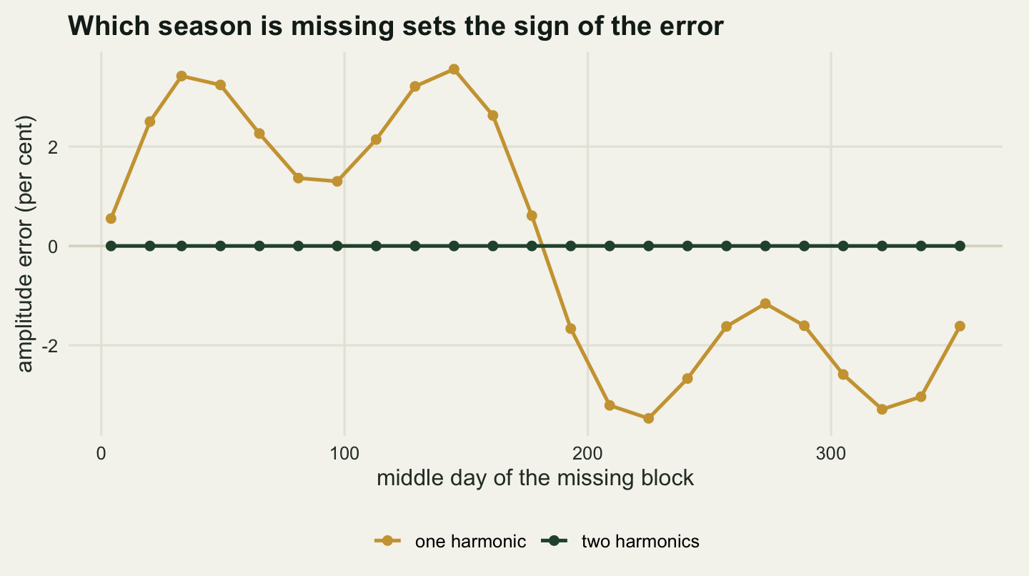
With one harmonic the same gap produces a bias. On the complete year the omitted second harmonic was orthogonal to the retained columns and cost nothing: 0.047 per cent. Take out the spring and the amplitude comes back 3.27 per cent too high; take out the senescence instead and it comes back 3.38 per cent too low. Same number of observations, same noise, opposite sign of error, and the direction is set purely by which side of the crest is missing.
sweep_len <- 9
sweep_start <- seq(1, n_lyr, by = 2)
gap_sweep <- do.call(rbind, lapply(sweep_start, function(st) {
  drop_idx <- ((st - 1 + seq_len(sweep_len) - 1) %% n_lyr) + 1
  keep_i <- setdiff(seq_len(n_lyr), drop_idx)
  mid_day <- ((doy[st] + (sweep_len - 1) * (doy[2] - doy[1]) / 2 - 1) %% 365) + 1
  do.call(rbind, lapply(1:2, function(kk) {
    f <- fit_harm(kk, keep_i, sig_obs)
    data.frame(mid_day = mid_day, harmonics = kk,
               amp_rel_bias = 100 * mean(f$amp / amp_true - 1),
               frac_over = mean(f$amp > amp_true))
  }))
}))
gap_sweep <- gap_sweep[order(gap_sweep$harmonics, gap_sweep$mid_day), ]
s1 <- gap_sweep[gap_sweep$harmonics == 1, ]
worst_hi <- s1[which.max(s1$amp_rel_bias), ]
worst_lo <- s1[which.min(s1$amp_rel_bias), ]
s2 <- gap_sweep[gap_sweep$harmonics == 2, ]
print(round(s1[, c("mid_day", "amp_rel_bias", "frac_over")], 4))
mid_day amp_rel_bias frac_over
43 4 0.5518 0.5406
45 20 2.5044 1.0000
1 33 3.4227 1.0000
3 49 3.2428 1.0000
5 65 2.2642 1.0000
7 81 1.3671 1.0000
9 97 1.3013 1.0000
11 113 2.1440 1.0000
13 129 3.2139 1.0000
15 145 3.5604 1.0000
17 161 2.6277 0.8219
19 177 0.6098 0.5969
21 193 -1.6647 0.2087
23 209 -3.2104 0.0000
25 225 -3.4726 0.0000
27 241 -2.6704 0.0000
29 257 -1.6208 0.0000
31 273 -1.1601 0.0000
33 289 -1.6059 0.0000
35 305 -2.5881 0.0000
37 321 -3.2906 0.0000
39 337 -3.0361 0.0175
41 353 -1.6142 0.2894print(round(c(worst_over_pct = worst_hi$amp_rel_bias,
worst_over_at_day = worst_hi$mid_day,
worst_under_pct = worst_lo$amp_rel_bias,
worst_under_at_day = worst_lo$mid_day,
largest_two_harmonic_bias_pct = max(abs(s2$amp_rel_bias))), 4)) worst_over_pct worst_over_at_day
3.5604 145.0000
worst_under_pct worst_under_at_day
-3.4726 225.0000
largest_two_harmonic_bias_pct
0.0000 Sweeping the block of 9 missing composites right around the year, on the noiseless signal so that only the geometry is left, gives the whole picture. With one harmonic the relative amplitude bias runs from +3.56 per cent when the block is centred on day 145 to -3.47 per cent when it is centred on day 225, and at both extremes 100 per cent of pixels are pushed the same way. With two harmonics the largest bias anywhere in the sweep is 4.1e-14 per cent, which is zero to machine precision.
The mechanism generalises past this example. Least squares does not bias the coefficients of a correctly specified model whatever the design is, so every bias here is the projection of the part of the signal the model does not carry onto the columns it does. On a complete evenly spaced year that projection is exactly zero by orthogonality of the harmonic basis, which is why a model one term short can look harmless. Remove a contiguous block of dates, the columns stop being orthogonal over the retained set, and the missing term leaks into the retained ones with a sign that follows its own sign over the retained window. Missing the green-up removes the part of the year where the asymmetry pulls the curve down, so the fitted swing is too large; missing the senescence removes where it pushes the curve up, so the swing is too small.
That is the finding of this section, and it is unpleasant. The number of harmonics stops being a variance question and becomes a bias question the moment the missing dates cluster in a season, which is the normal case. Choosing the model order on a complete year, or on the fit statistics, says nothing about how it will behave on the pixels where the cloud sat.
The coefficients are estimates, and they have standard errors
The amplitude map is a covariate now. It will go into a species distribution model, a comparison of grazing compartments, a regression of bird abundance on seasonal productivity. What travels into that model is a single number per pixel, and that number came out of a regression with 46 observations and 5 parameters, so it has a standard error the map does not show. The amplitude is a nonlinear function of two coefficients, so the delta method supplies it. With \(V\) the covariance matrix of the fitted coefficients,
\[\operatorname{Var}(A) \approx \frac{a^2 V_{aa} + 2ab\,V_{ab} + b^2 V_{bb}}{a^2 + b^2}\]
and the same construction with the derivatives of \(\operatorname{atan2}\) gives the standard error of the phase.
resid_full <- obs_mat - cf2 %*% t(des2)
df_resid <- n_lyr - ncol(des2)
s2_pix <- rowSums(resid_full^2) / df_resid
xtx_inv <- solve(crossprod(des2))
v_aa <- xtx_inv["cos1", "cos1"]; v_bb <- xtx_inv["sin1", "sin1"]
v_ab <- xtx_inv["cos1", "sin1"]
a_hat <- cf2[, "cos1"]; b_hat <- cf2[, "sin1"]
var_amp <- s2_pix * (a_hat^2 * v_aa + 2 * a_hat * b_hat * v_ab +
                       b_hat^2 * v_bb) / amp_hat^2
se_amp <- sqrt(var_amp)
var_phase <- s2_pix * (b_hat^2 * v_aa - 2 * a_hat * b_hat * v_ab +
                         a_hat^2 * v_bb) / amp_hat^4
se_phase_days <- sqrt(var_phase) / omega

cover90 <- mean(abs(amp_err) < qt(0.95, df_resid) * se_amp)
print(round(c(median_se_amp = median(se_amp), min_se_amp = min(se_amp),
              max_se_amp = max(se_amp), actual_sd_of_amp_error = sd(amp_err),
              coverage_of_90pct_interval = cover90), 5))
median_se_amp min_se_amp
0.00823 0.00501
max_se_amp actual_sd_of_amp_error
0.01200 0.00829
coverage_of_90pct_interval
0.90625 print(round(c(median_rel_se_pct = 100 * median(se_amp / amp_hat),
min_rel_se_pct = 100 * min(se_amp / amp_hat),
max_rel_se_pct = 100 * max(se_amp / amp_hat),
median_se_phase_days = median(se_phase_days)), 4)) median_rel_se_pct min_rel_se_pct max_rel_se_pct
3.1205 1.5897 7.8691
median_se_phase_days
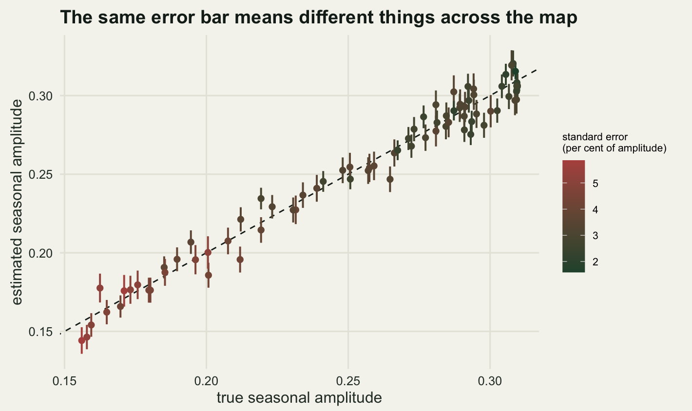
1.8271 The median per-pixel standard error on the amplitude is 0.00823, and the actual standard deviation of the amplitude error across the window is 0.00829, so the reported uncertainty is honest: a nominal 90 per cent interval covers the truth at 90.6 per cent of pixels. As a fraction of the amplitude being estimated it runs from 1.59 per cent in the closed canopy to 7.87 per cent over the thinnest grass, because the standard error is nearly constant across the window while the amplitude is not. The companion standard error on the phase has a median of 1.83 days.
That heterogeneity is the reason to keep the standard error rather than admire it. A covariate measured with error attenuates the coefficient it carries, by the reliability ratio: the variance of the true covariate over the variance of the true covariate plus the measurement error variance.
grass_only <- wood < 0.15
rel_all <- var(amp_true) / (var(amp_true) + mean(var_amp))
rel_grass <- var(amp_true[grass_only]) /
  (var(amp_true[grass_only]) + mean(var_amp[grass_only]))

print(round(c(pixels_all = n_cell, pixels_grass = sum(grass_only),
              sd_true_amp_all = sd(amp_true),
              sd_true_amp_grass = sd(amp_true[grass_only])), 5))
pixels_all pixels_grass sd_true_amp_all sd_true_amp_grass
1.600e+03 1.230e+02 5.324e-02 9.800e-03 print(round(c(reliability_all = rel_all,
attenuation_pct_all = 100 * (1 - rel_all),
reliability_grass = rel_grass,
attenuation_pct_grass = 100 * (1 - rel_grass)), 4)) reliability_all attenuation_pct_all reliability_grass
0.9763 2.3715 0.5763
attenuation_pct_grass
42.3727 Over the whole window the reliability ratio is 0.9763, so a slope fitted on the amplitude map would be attenuated by about 2.37 per cent. That sounds like permission to ignore the problem, and it is not, because the ratio is a property of the sample and not of the method. Restrict the analysis to the 123 grassland pixels, where the true amplitude has a standard deviation of 0.00980 instead of 0.05324, and the reliability falls to 0.5763: an attenuation of 42.4 per cent, enough to turn a real effect into a marginal one. The measurement error did not change. The contrast asked of it did.
Carrying the point estimate forward on its own treats a noisy quantity as known. The cheap partial fix is to carry se_amp alongside amp_hat, so the downstream model can at least weight the pixels, or report the reliability ratio and the attenuation. What that will not fix is a bias like the one in the previous section, which no standard error describes.
The honest limit
The truth here was generated as a sum of two harmonics and then fitted with harmonics, which is the friendliest possible case and inflates every recovery number above. The amplitude came back to 2.21 per cent and the peak day to 3 days because the model could represent the signal exactly. On real reflectance it never can, so the errors reported here are lower bounds. The one place the simulation was not friendly is the section on missing dates, where a model one term short of the truth was fitted on purpose, and that is exactly where the amplitude picked up a bias. The peak day has a bias of its own on the complete year, about 9.5 days, if you read it off the phase of the first harmonic instead of the fitted curve.
The harmonic form itself is a strong assumption. A single cosine is symmetric about its crest, which no growing season is. Two harmonics can lean but they cannot produce a fast green-up followed by a long slow senescence and a flat winter, which is the actual shape of a deciduous canopy, and pushing the order up to get it runs into the result of the harmonics section: more terms fit the noise and move the peak. A genuine double season is the worse case, because a low order fit to two peaks does not fail loudly. It returns a single smooth hump somewhere between them, with a plausible amplitude and a peak day corresponding to nothing that happened on the ground, and nothing in the residuals of a 40 by 40 window at this noise level would make that obvious. The general warning has been measured on real data: Atkinson, Jeganathan, Dash and Atzberger (2012) compared four smoothing models, harmonic analysis among them, and found the estimated dates depend on which was used, while White and colleagues (2009) put a number on it for North America, where ten methods on the same record gave mean start-of-spring dates spanning around three weeks, with the disagreement varying by land cover. A peak day is a property of a fitted curve, and the curve is a choice.
The gap analysis used contiguous blocks of missing dates, a caricature of what cloud does. Real masks are patchy, differ from pixel to pixel within a scene, and lose observations at a rate correlated with the surface state, so the missingness is not ignorable the way the random-drop scenario assumed: the direction of the bias should carry over, the size should not be read across. And nothing here has atmospheric correction, sensor drift, changing view geometry or georegistration error in it, the cube having arrived calibrated and aligned. Each of those can put a seasonal or spatial pattern into the coefficients that has nothing to do with vegetation, and a sub-pixel misregistration in particular puts a false amplitude signal along every land cover boundary, which is where the interesting ecology usually is.
Where to go next
The three coefficient rasters produced here, mean, amplitude and peak day, are covariates, and the checking post is the next step before they go anywhere: whether they vary enough to be worth modelling, and whether their errors are spatially correlated, are questions nothing above answers. If the missing dates in your own cube are the problem rather than a sideshow, the gap-filling post treats reconstruction properly. And if what you want is a phenological date to set against ground records, the phenology posts are where that comparison happens, with the warning from here attached: the satellite date and the observer date are two different measurements of a partly shared thing.
References
Jakubauskas ME, Legates DR, Kastens JH 2002 Computers and Electronics in Agriculture 37(1-3):127-139 (10.1016/S0168-1699(02)00116-3)
Roerink GJ, Menenti M, Verhoef W 2000 International Journal of Remote Sensing 21(9):1911-1917 (10.1080/014311600209814)
Zhang X, Friedl MA, Schaaf CB, Strahler AH, Hodges JCF, Gao F, Reed BC, Huete A 2003 Remote Sensing of Environment 84(3):471-475 (10.1016/S0034-4257(02)00135-9)
White MA, de Beurs KM, Didan K, et al 2009 Global Change Biology 15(10):2335-2359 (10.1111/j.1365-2486.2009.01910.x)
Verbesselt J, Hyndman R, Newnham G, Culvenor D 2010 Remote Sensing of Environment 114(1):106-115 (10.1016/j.rse.2009.08.014)
Atkinson PM, Jeganathan C, Dash J, Atzberger C 2012 Remote Sensing of Environment 123:400-417 (10.1016/j.rse.2012.04.001)
Zhu Z, Woodcock CE 2014 Remote Sensing of Environment 144:152-171 (10.1016/j.rse.2014.01.011)
Fisher NI 1993 Statistical Analysis of Circular Data. Cambridge University Press. ISBN 978-0-521-56890-6.