NDVI time series from a raster stack

Building a 46 layer NDVI cube in terra, the vector recycling trap that silently makes 1600 layers, per-pixel phenology with app, and how far a peak date drifts.

A mosaic of grassland and deciduous woodland, mapped for a grazing study, and a question about when each patch reaches its seasonal maximum of greenness. The satellite archive gives one eight-day composite of the normalised difference vegetation index per period, so forty-six images for a calendar year, and the window that has to be analysed is forty by forty pixels at thirty metres, twelve hundred metres on a side. That window is small on purpose: everything in this post has to run on a laptop while you read it, and the memory arithmetic at the end says what a realistic window would cost instead.

Forty-six images of the same sixteen hundred pixels is not forty-six maps. It is sixteen hundred time series, each one forty-six observations long, stored in the shape of a map. That difference sounds like bookkeeping and it is not: it changes which axis your code recycles along, which summaries make sense, and what a number pulled out of the cube actually estimates. The vegetation index itself is old and simple, a contrast between red and near infrared reflectance introduced by Tucker (1979), and its use as an ecological covariate is well trodden ground (Pettorelli et al 2005). The part that goes wrong is almost never the index. It is the layer axis.

This post sits alongside raster data in R with terra and repeats none of it. That post treats a raster as a map: one layer, an extent, a reference system, arithmetic between layers, slope off an elevation model, coarsening the grain, and reading values at sampling points. Everything there is about the two spatial dimensions. Here the grid is fixed and the third dimension is the subject. A SpatRaster with forty-six layers and a date attached to each one is a different object to reason about, and almost every mistake below happens on the axis that post never had.

Six things get measured. How a cube is built so that its time axis is a property of the object rather than a naming convention. What happens when a per-pixel vector meets a cube in an arithmetic expression, which is the single most useful paragraph here. What app() costs and buys against a loop over cells. How a series comes out of the cube at a point and how a per-pixel statistic goes back in as a layer. How far the date of maximum NDVI, the most popular of all land surface phenology metrics, sits from a known truth once compositing and noise have had their say. And where the cube lives in memory, with the two lines that tell you which mode you are in.

library(ggplot2)

te_pal <- list(forest = "#275139", green = "#2f8f63", sage = "#93a87f",
               clay = "#b5534e", gold = "#cda23f", line = "#dad9ca",
               ink = "#16241d", paper = "#f5f4ee")

theme_te <- function() {
  theme_minimal(base_size = 12) +
    theme(panel.grid.minor = element_blank(),
          panel.grid.major = element_line(colour = "#e7e6dc"),
          plot.background = element_rect(fill = "#f5f4ee", colour = NA),
          panel.background = element_rect(fill = "#f5f4ee", colour = NA),
          plot.title = element_text(face = "bold", colour = te_pal$ink),
          axis.title = element_text(colour = "#2c3a31"),
          axis.text = element_text(colour = "#2c3a31"))
}

A window with a known answer

The cube is simulated, and it is simulated because every claim below needs a verdict. Each pixel gets a seasonal NDVI curve with a baseline, an amplitude, a peak day and two widths, and those four quantities are written down before any observation exists. The peak day in particular is an exact property of the generating curve, so the error of an estimated peak day is a distance from a number that was set rather than an argument about what should have happened.

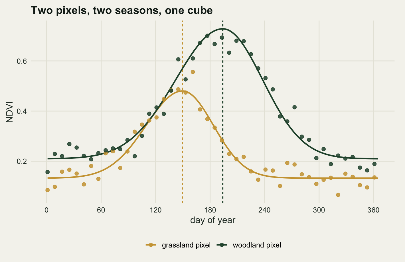
Two cover types share the window. Grassland greens up early, peaks in midsummer and senesces quickly under drought. Deciduous woodland leafs out later, reaches a higher amplitude and holds it for longer. The woodland patches are placed by thresholding a smoothed random field added to a broad trend, so the mosaic has irregular edges rather than a geometric pattern. On top of that sits a west to east moisture gradient that shifts the peak later and raises the amplitude as you move east, plus a small per-pixel departure so that no two pixels share a peak day exactly.

library(terra)
terraOptions(progress = 0)

n_side <- 40
n_lyr <- 46
pix_m <- 30
comp_days <- 8
doy <- seq(1, by = comp_days, length.out = n_lyr)
n_cell <- n_side^2

# cell centres in relative units; terra fills row-major from the top left
gx <- rep((seq_len(n_side) - 0.5) / n_side, times = n_side)
gy <- rep(rev((seq_len(n_side) - 0.5) / n_side), each = n_side)

box_smooth <- function(mm, rad) {
  nr <- nrow(mm)
  nc <- ncol(mm)
  acc <- matrix(0, nr, nc)
  for (dr in -rad:rad) for (dc in -rad:rad) {
    acc <- acc + mm[pmin(pmax(seq_len(nr) + dr, 1), nr),
                    pmin(pmax(seq_len(nc) + dc, 1), nc)]
  }
  acc / (2 * rad + 1)^2
}

set.seed(1207)
rough <- as.vector(box_smooth(matrix(rnorm(n_cell), n_side, n_side), 3))
wood_field <- sin(2.4 * pi * gx) * cos(1.8 * pi * gy) + 0.5 * gy +
  1.5 * rough / sd(rough)
is_wood <- wood_field > quantile(wood_field, 0.55)
moist <- 2 * (gx - 0.5)

set.seed(20260803)
pk_jitter <- rnorm(n_cell, 0, 4)
base_v <- ifelse(is_wood, 0.22, 0.15) + 0.02 * moist
amp_v <- ifelse(is_wood, 0.55, 0.40) + 0.06 * moist
peak_v <- ifelse(is_wood, 205, 165) + 18 * moist + pk_jitter
w_up <- ifelse(is_wood, 52, 40)
w_dn <- ifelse(is_wood, 44, 34)

season_at <- function(tt, b, a, p, wu, wd) {
  wid <- ifelse(tt < p, wu, wd)
  b + a * exp(-0.5 * ((tt - p) / wid)^2)
}
truth_mat <- outer(seq_len(n_cell), doy, function(i, dd)
  season_at(dd, base_v[i], amp_v[i], peak_v[i], w_up[i], w_dn[i]))

sd_obs <- 0.035
set.seed(4021)
ndvi_mat <- truth_mat + rnorm(length(truth_mat), 0, sd_obs)

print(c(pixels = n_cell, layers = n_lyr, window_m = n_side * pix_m,
        composite_days = comp_days, first_doy = doy[1], last_doy = doy[n_lyr]))

        pixels         layers       window_m composite_days      first_doy 
          1600             46           1200              8              1 
      last_doy 
           361 

print(round(c(woodland_fraction = mean(is_wood),
              mean_peak_grass = mean(peak_v[!is_wood]),
              mean_peak_wood = mean(peak_v[is_wood]),
              peak_min = min(peak_v), peak_max = max(peak_v),
              peak_sd = sd(peak_v), obs_noise_sd = sd_obs), 4))

woodland_fraction   mean_peak_grass    mean_peak_wood          peak_min 
           0.4500          166.4731          203.0908          137.9302 
         peak_max           peak_sd      obs_noise_sd 
         228.3061           21.3091            0.0350 

The window holds 1600 pixels of 30 metres, 45 per cent of them woodland, observed on 46 dates 8 days apart from day 1 to day 361. True peak days run from 137.9 to 228.3, a spread of 21.31 days, with grassland peaking around day 166.5 and woodland around day 203.1. Observation noise has a standard deviation of 0.035 NDVI units, which is the sort of residual scatter an eight-day composite carries after the worst cloud has been screened out.

The time axis is a property, not a naming convention

A cube is built the same way a single layer is, with one extra argument. nlyrs sets the depth, values() fills it from a matrix of one row per pixel and one column per layer, and time() attaches a real date to each layer.

cube <- rast(nrows = n_side, ncols = n_side, nlyrs = n_lyr,
             xmin = 412000, xmax = 412000 + n_side * pix_m,
             ymin = 5050000, ymax = 5050000 + n_side * pix_m,
             crs = "EPSG:32634")
values(cube) <- ndvi_mat
time(cube) <- as.Date("2024-01-01") + doy - 1
names(cube) <- paste0("d", formatC(doy, width = 3, flag = "0"))
cube

class       : SpatRaster
size        : 40, 40, 46  (nrow, ncol, nlyr)
resolution  : 30, 30  (x, y)
extent      : 412000, 413200, 5050000, 5051200  (xmin, xmax, ymin, ymax)
coord. ref. : WGS 84 / UTM zone 34N (EPSG:32634)
source(s)   : memory
names       :     d001,     d009,     d017,     d025,     d033,     d041, ...
min values  : 0.045825, 0.036902, 0.034353, 0.022009, 0.053039, 0.026604, ...
max values  : 0.328978, 0.353429, 0.319029, 0.324503, 0.378971, 0.337148, ...
time (days) : 2024-01-01 to 2024-12-26 (46 steps)

The printout carries a line the single-layer version does not have. Alongside the dimensions, the resolution, the extent and the reference system there is now a time range, and that range is stored with the object rather than parsed out of layer names when somebody needs it. The distinction matters the first time a subset is taken: cube[[10:20]] keeps the right eleven dates without anyone having to think about it, and a layer name of d073 is a label while time() is data.

print(c(layers = nlyr(cube), cells = ncell(cube),
        values_total = ncell(cube) * nlyr(cube)))

      layers        cells values_total 
          46         1600        73600 

print(head(time(cube), 4))

[1] "2024-01-01" "2024-01-09" "2024-01-17" "2024-01-25"

print(range(time(cube)))

[1] "2024-01-01" "2024-12-26"

print(table(as.numeric(diff(time(cube)))))

 8 
45 

sub_cube <- cube[[10:20]]
print(c(sub_layers = nlyr(sub_cube)))

sub_layers 
        11 

print(range(time(sub_cube)))

[1] "2024-03-13" "2024-06-01"

nlyr() returns 46 and ncell() returns 1600, so the object holds 73,600 values. Every gap between consecutive dates is 8 days, which is worth checking on a real archive rather than assuming: a composite series with a missing period has an irregular time axis, and any code that treats layer index as time will be wrong from that layer onwards. The eleven layer subset keeps its dates, running from 2024-03-13 to 2024-06-01.

The trap: a bare vector plus a cube

Here is the mistake this post exists for. Suppose a topographic correction has been worked out per pixel: one number for each of the 1600 cells, to be added to every layer. The expression that says that in English is cube + correction, and R will run it.

set.seed(3311)
topo_adj <- runif(n_cell, -0.02, 0.02)
trap <- cube + topo_adj

print(c(input_layers = nlyr(cube), correction_length = length(topo_adj),
        output_layers = nlyr(trap), output_cells = ncell(trap)))

     input_layers correction_length     output_layers      output_cells 
               46              1600              1600              1600 

print(c(time_all_missing = all(is.na(time(trap)))))

time_all_missing 
            TRUE 

# what each output layer actually did to the first three pixels
print(round(as.numeric(values(trap)[1:3, 1] - values(cube)[1:3, 1]), 5))

[1] 0.01684 0.01684 0.01684

print(round(as.numeric(values(trap)[1:3, 2] - values(cube)[1:3, 2]), 5))

[1] 0.01223 0.01223 0.01223

print(round(topo_adj[1:3], 5))

[1]  0.01684  0.01223 -0.01091

The cube went in with 46 layers and came out with 1600. No error, no warning, nothing in the console to look at. What terra did is defensible once you see it: in an arithmetic expression a bare numeric vector supplies one value per layer, not one value per cell, so a vector of length 1600 describes 1600 layers. The two operands are then recycled to the longer of the two, giving 1600 layers in which layer k is a layer of the cube plus the single constant topo_adj[k]. The differences printed above are the signature: subtract the original from output layer one and every pixel has moved by the same amount, the first entry of the correction vector, while output layer two has moved by the second entry. The dates go too. all(is.na(time(trap))) is TRUE, because 1600 layers cannot inherit 46 dates.

Nothing about this is exotic and nothing about it announces itself. A cube of 46 layers becomes a cube of 1600, the object still prints, still has an extent, still draws, and the next function in the pipeline receives something with the right class and the wrong shape. On a real cube with a real file behind it, the same expression can also start writing gigabytes to a temporary directory.

Two forms do what was intended. The first wraps the vector in a raster of the right geometry and lets terra broadcast it across layers; the second edits the value matrix directly and puts it back with setValues().

adj_layer <- setValues(cube[[1]], topo_adj)
fix_broadcast <- cube + adj_layer

fix_setvalues <- setValues(cube, values(cube) + topo_adj)

forms_agree <- all(values(fix_broadcast) == values(fix_setvalues))
print(c(broadcast_layers = nlyr(fix_broadcast),
        setvalues_layers = nlyr(fix_setvalues),
        two_forms_agree_exactly = forms_agree,
        dates_kept = identical(time(fix_broadcast), time(cube))))

       broadcast_layers        setvalues_layers two_forms_agree_exactly 
                     46                      46                       1 
             dates_kept 
                      1 

print(round(as.numeric(values(fix_broadcast)[1:3, 1] - values(cube)[1:3, 1]), 5))

[1]  0.01684  0.01223 -0.01091

print(round(as.numeric(values(fix_broadcast)[1:3, 2] - values(cube)[1:3, 2]), 5))

[1]  0.01684  0.01223 -0.01091

Both return 46 layers, the two forms agree cell for cell, and the broadcast form keeps the dates. The first three pixels now carry three different offsets, and those offsets are the same in layer one as in layer two, which is what a per-pixel correction is supposed to look like. Note that values(cube) + topo_adj works because the value matrix is 1600 by 46 and R recycles a length 1600 vector down the columns; that is ordinary matrix recycling and it is a different rule from the one terra applies to the raster.

The habit that catches all of this is one line long. After any arithmetic you did not write carefully, check nlyr(). If the answer is not the number you started with, or a number you deliberately asked for, stop there. It costs nothing and it is the only cheap test for a class of error that produces no message at all.

Per-pixel summaries with app

The natural summaries of a cube run down the layer axis: the annual mean of each pixel, the seasonal amplitude of each pixel, the layer at which each pixel is largest. app() applies a function to the vector of layer values at every cell and returns a raster with as many layers as the function returns values.

mean_r <- app(cube, mean)
names(mean_r) <- "annual_mean"

amp_r <- app(cube, function(x) max(x) - min(x))
names(amp_r) <- "range_ndvi"

argmax_r <- app(cube, which.max)
peak_raw_r <- setValues(argmax_r, doy[values(argmax_r)[, 1]])
names(peak_raw_r) <- "peak_doy_raw"

print(c(mean_layers = nlyr(mean_r), amp_layers = nlyr(amp_r)))

mean_layers  amp_layers 
          1           1 

print(round(global(c(mean_r, amp_r, peak_raw_r), c("mean", "range")), 4))

                 mean      min      max
annual_mean    0.3176   0.2057   0.4459
range_ndvi     0.5576   0.3803   0.7752
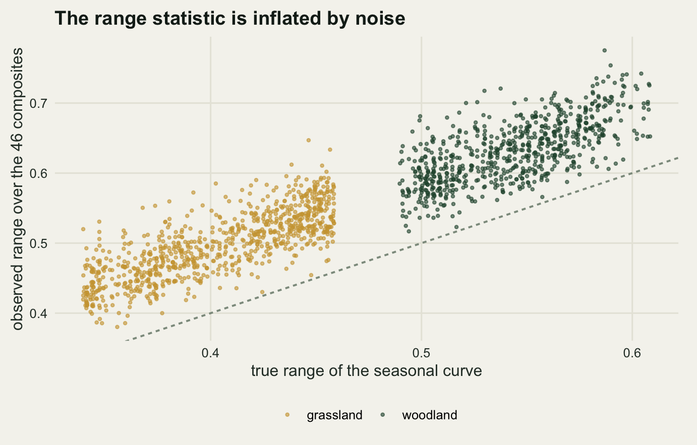
peak_doy_raw 181.2750 121.0000 241.0000

Each summary collapses 46 layers to one, so the output has 1 layer and the same 1600 cells. Mean annual NDVI over the window is 0.3176, and the observed range within a pixel averages 0.5576.

That second number needs a warning attached, and it is a good example of a summary that is easy to compute and easy to misread. The observed range is the maximum of 46 noisy values minus the minimum of the same 46, so noise pushes the maximum up and the minimum down and the statistic is biased away from zero whatever the truth is.

amp_obs <- values(amp_r)[, 1]
amp_true <- apply(truth_mat, 1, max) - apply(truth_mat, 1, min)
amp_gap <- amp_obs - amp_true

print(round(c(mean_observed_range = mean(amp_obs),
              mean_true_range = mean(amp_true),
              mean_inflation = mean(amp_gap),
              pct_inflation = 100 * mean(amp_obs / amp_true - 1),
              share_overestimated = mean(amp_gap > 0),
              obs_noise_sd = sd_obs), 4))

mean_observed_range     mean_true_range      mean_inflation       pct_inflation 
             0.5576              0.4667              0.0909             20.1310 
share_overestimated        obs_noise_sd 
             1.0000              0.0350 

The observed range averages 0.5576 against a true sampled amplitude of 0.4667, an inflation of 0.0909 NDVI units or 20.13 per cent, and it is too large in 100 per cent of pixels. The inflation is 2.6 times the observation standard deviation, which is what order statistics predict: the largest of the handful of composites near the seasonal peak sits above the curve, the smallest of the winter composites sits below it, and the two displacements add. Any comparison of amplitude between two cubes with different noise levels, two sensors say, is partly a comparison of their noise. A difference between two percentiles is the cheap fix, and it is not free either: it shrinks the estimate towards the middle of the season.

Now the timing question, because the loop over cells is the first thing most people write.

n_time <- 20
t_app <- system.time(for (k in seq_len(n_time)) app(cube, mean))[["elapsed"]] / n_time
t_naive <- system.time({
  naive_mean <- vapply(seq_len(ncell(cube)),
                       function(i) mean(unlist(cube[i])), numeric(1))
})[["elapsed"]]
t_matrix <- system.time(for (k in seq_len(n_time))
  rowMeans(values(cube)))[["elapsed"]] / n_time

print(round(c(app_ms = 1000 * t_app, cell_loop_ms = 1000 * t_naive,
              matrix_ms = 1000 * t_matrix), 3))

      app_ms cell_loop_ms    matrix_ms 
        1.10      1354.00         0.35 

print(round(c(loop_over_app = t_naive / t_app,
              app_over_matrix = t_app / t_matrix), 2))

  loop_over_app app_over_matrix 
        1230.91            3.14 

print(c(app_matches_loop = max(abs(values(mean_r)[, 1] - naive_mean)),
        app_matches_matrix = max(abs(values(mean_r)[, 1] - rowMeans(values(cube))))))

  app_matches_loop app_matches_matrix 
      2.775558e-16       0.000000e+00 

All three agree to floating point, the largest disagreement being 2.78e-16. The times do not agree at all. app() takes 1.1 milliseconds, the loop over cells takes 1354 milliseconds, a factor of 1231. The loop is slow for a reason that has nothing to do with R being slow at loops: cube[i] is a fresh indexed read of the raster, so the loop performs 1600 separate reads where app() performs one pass.

The third row is the honest one. Pulling the whole cube into a matrix with values() and calling rowMeans() takes 0.35 milliseconds, so app() costs 3.14 times that on a window this small. At 1600 pixels the difference between the two sensible options is a rounding error and either is fine. It stops being a rounding error at the point where values() no longer fits: app() is written to work chunk by chunk, so it keeps working when the matrix approach fails outright, and that crossover is what the last section measures.

Figure 1: Mean annual NDVI over the 40 by 40 pixel window, with the six sampling points marked. The woodland patches carry the higher annual mean and form irregular blocks around the edges of the window; the grassland between them is paler. Averaging 46 layers down to one number per pixel leaves almost no visible grain, which is why the mean is the easiest summary to trust and the peak date is the hardest.

Figure 2: Observed within-pixel range of NDVI against the true range of the underlying seasonal curve at the same 46 dates, one point per pixel. The dashed line is equality. Every point sits above it, because the maximum of a noisy series is biased up and the minimum is biased down, and the vertical offset is close to constant across the whole amplitude gradient and across both cover types.

Out of the cube at a point, and back in as a layer

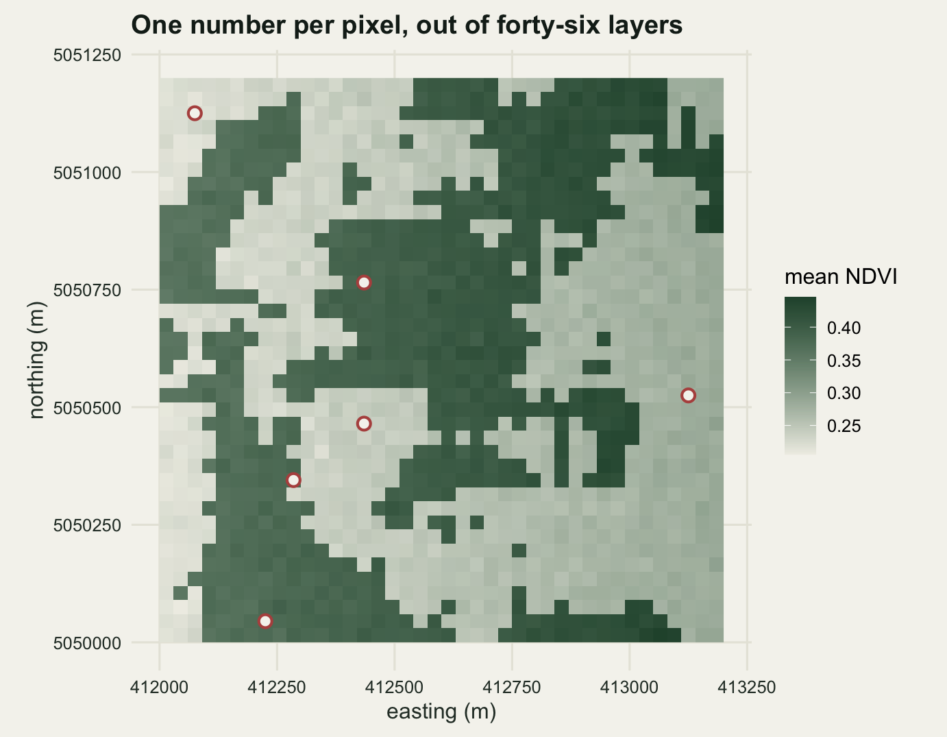
The other direction is the one field ecologists reach for: a handful of monitoring plots with coordinates, and a request for the NDVI series at each. extract() takes the cube and a SpatVector of points and returns one row per point with one column per layer, which is a wide table rather than a long one.

pts <- vect(as.matrix(pt_xy), type = "points", crs = crs(cube))
ex <- extract(cube, pts)

print(dim(ex))

[1]  6 47

print(round(as.matrix(ex[1:3, 2:6]), 4))

    d001   d009   d017   d025   d033
1 0.0845 0.0976 0.1580 0.1658 0.1506
2 0.1693 0.1944 0.1720 0.1104 0.1251
3 0.1341 0.1518 0.1547 0.2221 0.1938

ser_long <- data.frame(
  point = rep(seq_len(nrow(ex)), each = n_lyr),
  doy = rep(doy, times = nrow(ex)),
  ndvi = as.numeric(t(as.matrix(ex[, -1]))),
  cover = rep(ifelse(is_wood[pt_cells], "woodland", "grassland"),
              each = n_lyr))
print(round(tapply(ser_long$ndvi, ser_long$cover, mean), 4))

grassland  woodland 
   0.2491    0.3816 

print(c(cells_hit = identical(as.integer(cellFromXY(cube, as.matrix(pt_xy))),
                              as.integer(pt_cells))))

cells_hit 
     TRUE 

The returned table is 6 rows by 47 columns: an ID column plus one column per layer, named from the layer names rather than from time(), which is the first reason to keep time() in the object and reattach it after extraction. The six points fall on the cells they were drawn from, and the woodland points average 0.3816 against 0.2491 for grassland across the whole year.

Figure 3: Annual NDVI at two contrasting pixels, one grassland and one deciduous woodland, from the same cube. Dots are the 46 eight-day composites, the solid line is the generating seasonal curve evaluated daily, and the dashed vertical lines mark the true peak day of each pixel. The woodland curve peaks about forty-five days later, reaches a higher maximum and holds it longer, and the scatter of the dots around each curve is the observation noise that every peak-date estimator has to work through.

The round trip is the other half. A statistic computed as a plain vector, one value per pixel, becomes a raster layer by handing it to setValues() with a single-layer template taken from the cube. That template is what carries the geometry: the same number of cells in the same order, the same extent, the same resolution and the same reference system.

fastest_rise <- function(x) max(diff(x)) / comp_days
grow_obs <- apply(ndvi_mat, 1, fastest_rise)
grow_true <- apply(truth_mat, 1, fastest_rise)

rate_r <- setValues(cube[[1]], grow_obs)
names(rate_r) <- "max_greenup_rate"

print(c(is_plain_vector = is.numeric(grow_obs),
        vector_length = length(grow_obs),
        raster_layers = nlyr(rate_r), raster_cells = ncell(rate_r)))

is_plain_vector   vector_length   raster_layers    raster_cells 
              1            1600               1            1600 

print(c(same_extent = identical(as.vector(ext(rate_r)), as.vector(ext(cube))),
        same_res = identical(res(rate_r), res(cube)),
        same_crs = identical(crs(rate_r), crs(cube))))

same_extent    same_res    same_crs 
       TRUE        TRUE        TRUE 

print(round(c(mean_observed_rate = mean(grow_obs),
              mean_true_rate = mean(grow_true),
              ratio_observed_to_true = mean(grow_obs) / mean(grow_true),
              observed_above_true = mean(grow_obs > grow_true)), 4))

    mean_observed_rate         mean_true_rate ratio_observed_to_true 
                0.0158                 0.0062                 2.5456 
   observed_above_true 
                1.0000 

The vector had 1600 entries and the layer has 1600 cells in the same order, with the extent, resolution and reference system inherited from the template. The statistic itself is a warning repeated. The fastest observed rise averages 0.01578 NDVI units per day against a true 0.0062, a factor of 2.55, and it is too steep in 100 per cent of pixels. A difference between two consecutive noisy observations carries the noise of both, and taking the largest of 45 such differences selects for the pair where the noise happened to help. Green-up rate read off raw composites is mostly a measurement of the noise floor.

The wrong way to build the same layer is cube[[1]] * 0 + grow_obs, which looks harmless and lands straight back in the trap from two sections ago.

How far off is the peak date

The date of maximum NDVI is the most heavily used land surface phenology metric there is, and the reason is that it takes one line. Its long history in satellite phenology runs from Reed et al (1994), who set out the family of metrics that can be pulled from an annual NDVI trajectory, through the curve-fitting approach of Zhang et al (2003) built for MODIS. What it costs is worth measuring, and the measurement here is clean because the true peak day of every pixel is known to a fraction of a day.

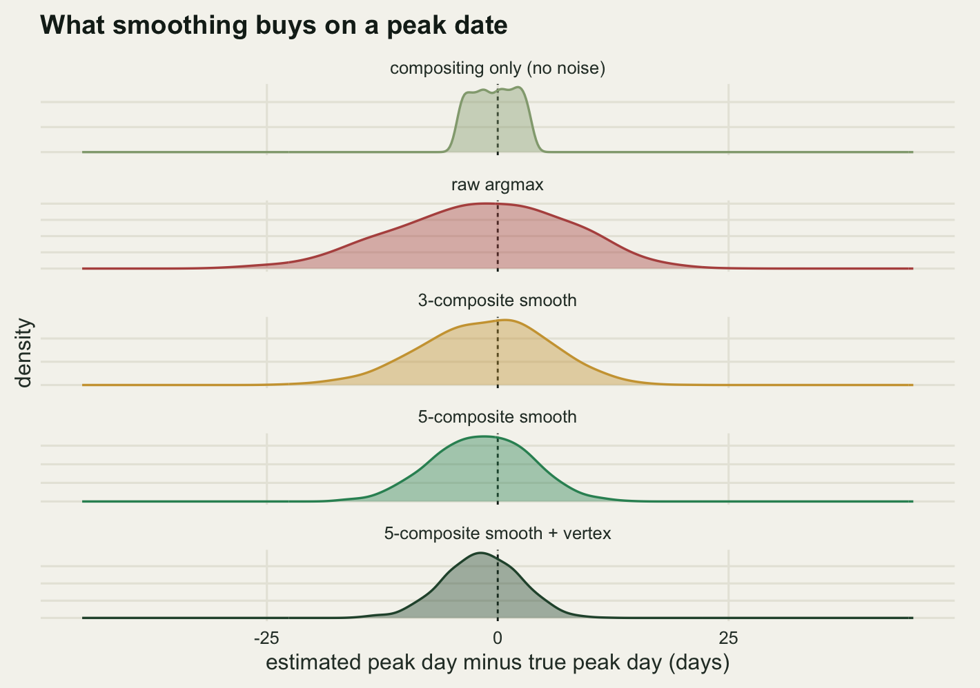
Four estimators are compared. The first is the argmax of the raw composites, quantised to the 8 day grid. The second smooths each series with a moving average of three composites before taking the argmax, the third with five. The fourth takes the five-composite smooth, finds its argmax, then fits a parabola through that point and its two neighbours and uses the vertex, which gives a continuous date rather than one of 46 grid values. There is also a floor: the argmax of the noise-free curve sampled at the same 46 dates, which is what compositing alone costs before any noise is added.

smooth_k <- function(x, k) {
  half <- (k - 1) / 2
  n <- length(x)
  vapply(seq_len(n),
         function(j) mean(x[max(1, j - half):min(n, j + half)]),
         numeric(1))
}

argmax_doy <- function(M) doy[max.col(M, ties.method = "first")]

vertex_offset <- function(y, j) {
  n <- length(y)
  if (j <= 1 || j >= n) return(0)
  den <- y[j - 1] - 2 * y[j] + y[j + 1]
  if (den >= 0) return(0)
  0.5 * (y[j - 1] - y[j + 1]) / den
}

sm3_mat <- t(apply(ndvi_mat, 1, smooth_k, k = 3))
sm5_mat <- t(apply(ndvi_mat, 1, smooth_k, k = 5))
j5 <- max.col(sm5_mat, ties.method = "first")
off5 <- vapply(seq_len(n_cell),
               function(i) vertex_offset(sm5_mat[i, ], j5[i]), numeric(1))

pk_floor <- argmax_doy(truth_mat)
pk_rawmax <- argmax_doy(ndvi_mat)
pk_ma3 <- argmax_doy(sm3_mat)
pk_ma5 <- argmax_doy(sm5_mat)
pk_par <- doy[j5] + comp_days * off5

print(round(c(vertex_offset_min = min(off5), vertex_offset_max = max(off5),
              offsets_at_zero = sum(off5 == 0)), 4))

vertex_offset_min vertex_offset_max   offsets_at_zero 
          -0.4988            0.4997            0.0000 

The vertex offsets stay inside plus or minus half a composite interval, as they must, and none of the 1600 pixels fell back on the zero offset that guards against a maximum at the end of the series or a locally convex triple.

err_row <- function(v) c(rmse = sqrt(mean((v - peak_v)^2)),
                         mae = mean(abs(v - peak_v)),
                         bias = mean(v - peak_v),
                         within_8 = mean(abs(v - peak_v) <= 8),
                         within_16 = mean(abs(v - peak_v) <= 16))
pk_tab <- rbind(compositing_only = err_row(pk_floor),
                raw_argmax = err_row(pk_rawmax),
                smooth_3 = err_row(pk_ma3),
                smooth_5 = err_row(pk_ma5),
                smooth_5_vertex = err_row(pk_par))
print(round(pk_tab, 4))

                   rmse    mae    bias within_8 within_16
compositing_only 2.3604 2.0361 -0.3511   1.0000    1.0000
raw_argmax       9.3323 7.5245 -1.6761   0.5956    0.9219
smooth_3         6.9098 5.5136 -1.3461   0.7550    0.9769
smooth_5         5.5029 4.4160 -1.7511   0.8569    0.9969
smooth_5_vertex  4.4929 3.5775 -1.7724   0.9244    1.0000

mc_se <- sd((pk_par - peak_v)^2) / sqrt(n_cell) / (2 * pk_tab["smooth_5_vertex", "rmse"])
print(round(c(rmse_drop_days = pk_tab["raw_argmax", "rmse"] -
                pk_tab["smooth_5_vertex", "rmse"],
              rmse_drop_pct = 100 * (1 - pk_tab["smooth_5_vertex", "rmse"] /
                                       pk_tab["raw_argmax", "rmse"]),
              monte_carlo_se_days = mc_se), 4))

     rmse_drop_days       rmse_drop_pct monte_carlo_se_days 
             4.8394             51.8566              0.0815 

print(round(rbind(
  raw = tapply(abs(pk_rawmax - peak_v), ifelse(is_wood, "wood", "grass"), mean),
  vertex = tapply(abs(pk_par - peak_v), ifelse(is_wood, "wood", "grass"), mean)), 4))

        grass   wood
raw    7.2113 7.9073
vertex 3.3366 3.8720

Compositing alone costs 2.36 days of root mean squared error. That is the floor, and it is close to the standard deviation of a uniform distribution over one 8 day interval, which is what quantising a continuous peak day to a grid of dates does. Nothing about the analysis can go below it while the observations arrive 8 days apart.

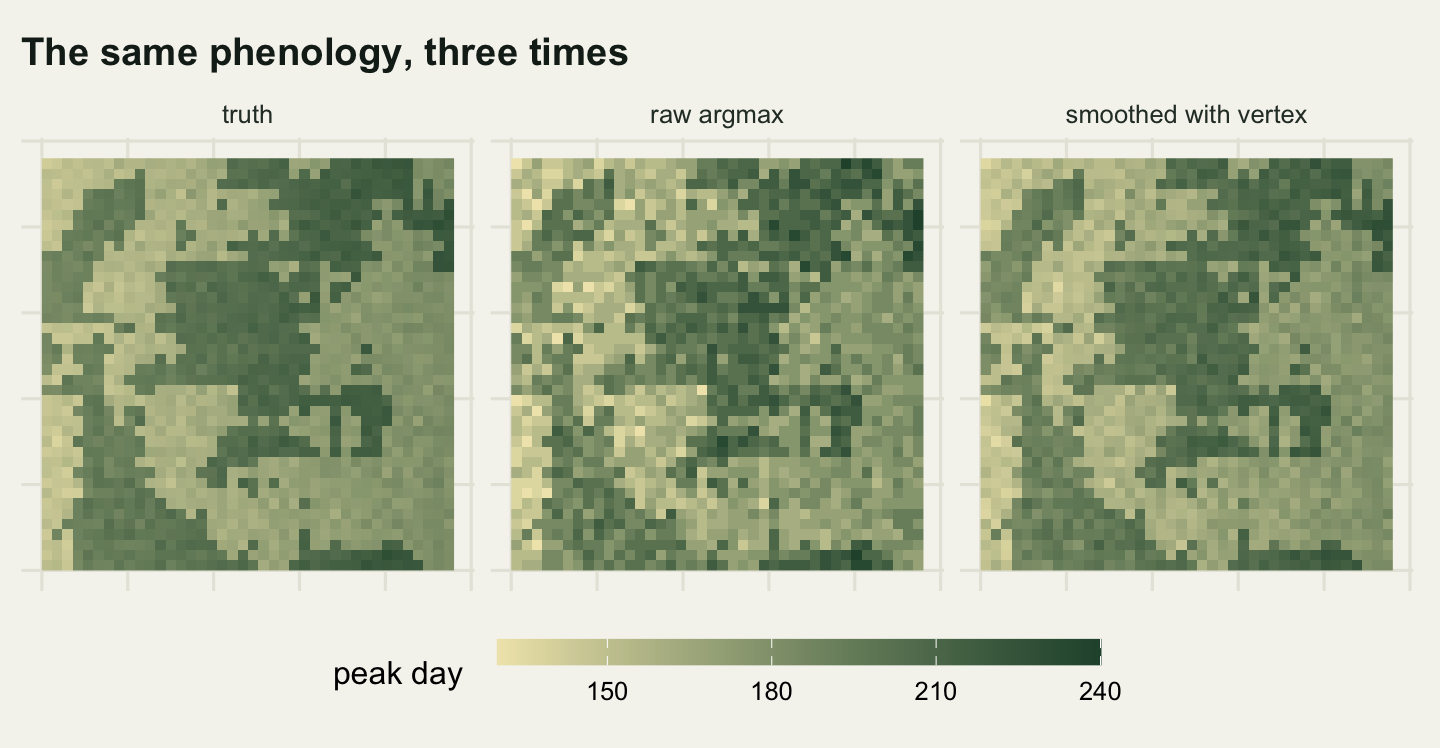
Noise takes the raw argmax to 9.33 days, 3.95 times the floor, with a mean absolute error of 7.52 days. Only 59.6 per cent of pixels land within one composite interval of the truth and 92.2 per cent within two. A map of raw argmax over this window would show pixel to pixel variation of that size on top of a real between-pixel spread of 21.31 days, so a large part of the texture in such a map is the noise rather than the vegetation.

Smoothing recovers most of it. A three-composite moving average brings the error to 6.91 days and five composites to 5.5. Adding the parabola vertex on top, which is the only step that escapes the 8 day grid, gives 4.49 days: a drop of 4.84 days, or 51.9 per cent, against a Monte Carlo standard error of 0.082 days on the final figure. The proportion within one composite interval goes from 59.6 to 92.4 per cent, and every pixel is now within two.

All five estimators carry a small negative bias, from -0.35 to -1.77 days. That is the asymmetry of the generating curve showing through: both cover types rise more slowly than they fall, so the broader flank sits before the peak and any estimator that leans on neighbouring composites is pulled that way. The bias is small against the scatter, which is why the root mean squared error and the mean absolute error tell the same story here. It does not shrink as the smoother widens, and between three composites and five it grows.

Woodland is harder than grassland at every stage. Mean absolute error for the raw argmax is 7.91 days in woodland against 7.21 in grassland, and after smoothing and the vertex it is 3.87 against 3.34. Its season is broader, so the curvature near the maximum is gentler and the same noise buys a bigger displacement. That is a general property rather than a fact about this simulation, and it is the reason peak-date maps look noisiest over exactly the vegetation whose season is longest.

The step from a moving average to a fitted seasonal curve is where the next post in this group starts. A harmonic model uses all 46 observations to estimate the shape rather than the five nearest to the maximum, and it returns a phase directly instead of an argmax; that is harmonic regression on a seasonal raster, and the comparison of extraction methods across North America in White et al (2009) is the reason to take the choice seriously rather than treating one metric as the answer.

Figure 4: Distribution of estimated minus true peak day over all 1600 pixels for four estimators, plus the floor set by eight-day compositing alone. The raw argmax is spread over more than a month and is quantised onto the composite grid. Smoothing narrows it, and the parabola vertex on the five-composite smooth removes the quantisation as well, ending closer to the compositing floor than to the raw estimator.

Figure 5: True peak day, the raw argmax estimate and the smoothed estimate with a parabola vertex, mapped over the same window. The woodland patches peak about forty days later than the grassland around them, and a west to east gradient shifts both. The raw argmax reproduces the pattern with heavy pixel to pixel speckle, including cells that look forty days out of place next to their neighbours; the smoothed estimate recovers most of the structure and leaves much less of the speckle.

Where the cube lives

A cube is either in memory or on disk, and terra decides which without asking. Two lines tell you where you stand.

cube_mb <- ncell(cube) * nlyr(cube) * 8 / 1024^2

print(c(in_memory = inMemory(cube), any_source_file = any(nchar(sources(cube)) > 0)))

      in_memory any_source_file 
           TRUE           FALSE 

print(round(c(values_held = ncell(cube) * nlyr(cube),
              megabytes_double = cube_mb,
              object_size_bytes = as.numeric(object.size(cube))), 3))

      values_held  megabytes_double object_size_bytes 
        73600.000             0.562          1304.000 

inMemory() returns TRUE and sources() gives an empty string, so every value is in RAM. The cube holds 73,600 numbers, which is 0.562 megabytes as double precision. Note the third figure: object.size() reports 1304 bytes for the same object, because a SpatRaster is an R wrapper around a C++ object and R cannot see through it. object.size() is the wrong tool here and will tell you a cube of any size is about a kilobyte.

When the values do not fit, terra writes the result of an operation to a temporary file and processes the input in horizontal blocks. That behaviour can be triggered deliberately by setting the memory ceiling low, which is the cheapest way to see what a real large-cube run does.

mean_disk <- local({
  terraOptions(memmax = 0.0001, memmin = 0.00001)
  on.exit(terraOptions(memmax = -1, memmin = 1))
  app(cube, mean)
})

disk_gap <- max(abs(as.numeric(values(mean_disk)) - as.numeric(values(mean_r))))
print(c(in_memory = inMemory(mean_disk),
        has_source_file = any(nchar(sources(mean_disk)) > 0),
        extension = tools::file_ext(sources(mean_disk))))

      in_memory has_source_file       extension 
        "FALSE"          "TRUE"           "tif" 

print(c(agree_to_six_digits =
          isTRUE(all.equal(as.numeric(values(mean_disk)),
                           as.numeric(values(mean_r)), tolerance = 1e-6))))

agree_to_six_digits 
               TRUE 

print(formatC(disk_gap, format = "e", digits = 3))

[1] "1.489e-08"

inMemory() now returns FALSE and sources() points at a tif file in the temporary directory. The answers agree with the in-memory version to 1.49e-08, and that gap is not zero: the default write is single precision, so a disk round trip drops the tail of the number. For NDVI that is irrelevant. For an accumulated sum over thousands of layers, or a difference between two nearly equal cubes, it may not be.

The arithmetic that decides which mode a real job lands in is worth doing before the job starts rather than after.

country_km2 <- 93030
scale_tab <- t(vapply(c(10, 30, 250, 1000), function(m_res) {
  px <- country_km2 * 1e6 / m_res^2
  c(resolution_m = m_res, million_pixels = px / 1e6,
    gb_one_layer = px * 8 / 1024^3,
    gb_46_layers = px * 46 * 8 / 1024^3)
}, numeric(4)))
print(round(scale_tab, 3))

     resolution_m million_pixels gb_one_layer gb_46_layers
[1,]           10        930.300        6.931      318.839
[2,]           30        103.367        0.770       35.427
[3,]          250          1.488        0.011        0.510
[4,]         1000          0.093        0.001        0.032

print(round(c(window_mb = cube_mb,
              windows_per_gb = 1024 / cube_mb), 1))

     window_mb windows_per_gb 
           0.6         1823.6 

A country of 93,030 square kilometres at 30 metres is 103.4 million pixels, so a year of 46 composites is 35.4 gigabytes at double precision, and at 10 metres it is 318.8 gigabytes. The window in this post is 0.562 megabytes: you could hold 1,824 of them in a gigabyte. That gap is the whole reason app() exists in the form it does, and it is the reason the answer to “why not just pull it into a matrix” is different at the two scales.

The honest limit

The cube is simulated, and the list of what a simulation of this kind leaves out is longer than the list of what it includes. There is no atmospheric correction here, so no residual aerosol or water vapour effect that varies between dates and biases whole composites in the same direction. There is no sensor drift, so no slow change in calibration that a long series would read as a trend in greenness. There is no bidirectional reflectance effect, so the view and illumination geometry that changes across a swath and through the season never touches the numbers; that is one of the effects the MODIS vegetation index products were designed around (Huete et al 2002). And there is no georegistration error between dates, so a pixel is the same patch of ground on every layer. Each of those is a real source of apparent phenological change, and each of them would inflate the peak-date errors measured above rather than shrink them.

The noise model is the weakest part. Observation errors here are independent between dates, and real composite errors are not: haze, thin cloud and snow persist for days, so an error in one composite predicts the error in the next. Replacing the independent noise with a first order autoregressive process at the same marginal standard deviation is a two-line change, and it is worth the two lines because it moves the answer.

rho_ar <- 0.5
set.seed(7788)
ar_mat <- matrix(0, n_cell, n_lyr)
e_prev <- rnorm(n_cell, 0, sd_obs)
ar_mat[, 1] <- e_prev
for (k in 2:n_lyr) {
  e_prev <- rho_ar * e_prev + rnorm(n_cell, 0, sd_obs * sqrt(1 - rho_ar^2))
  ar_mat[, k] <- e_prev
}
ndvi_ar <- truth_mat + ar_mat

sm5_ar <- t(apply(ndvi_ar, 1, smooth_k, k = 5))
j5_ar <- max.col(sm5_ar, ties.method = "first")
pk_par_ar <- doy[j5_ar] + comp_days *
  vapply(seq_len(n_cell),
         function(i) vertex_offset(sm5_ar[i, ], j5_ar[i]), numeric(1))

lag1_ar <- mean(vapply(seq_len(n_cell),
                       function(i) cor(ar_mat[i, -n_lyr], ar_mat[i, -1]),
                       numeric(1)))
print(round(c(marginal_sd = sd(ar_mat),
              mean_lag1_correlation = lag1_ar,
              raw_rmse_iid = pk_tab["raw_argmax", "rmse"],
              raw_rmse_ar = sqrt(mean((argmax_doy(ndvi_ar) - peak_v)^2)),
              vertex_rmse_iid = pk_tab["smooth_5_vertex", "rmse"],
              vertex_rmse_ar = sqrt(mean((pk_par_ar - peak_v)^2))), 4))

          marginal_sd mean_lag1_correlation          raw_rmse_iid 
               0.0349                0.4391                9.3323 
          raw_rmse_ar       vertex_rmse_iid        vertex_rmse_ar 
               9.3147                4.4929                5.0370 

The marginal standard deviation is unchanged at 0.0349, the mean lag-one correlation within a pixel is 0.439, and the raw argmax barely moves, from 9.33 days to 9.31. The smoothed estimator loses more: 4.49 days becomes 5.04, giving up 12.1 per cent, because a moving average cannot average away a disturbance it shares with its neighbours. The direction of that result is the point: every smoother in this post is flattered by independent noise, and the real thing is correlated.

Compositing itself is treated as a clean sampling of the curve every 8 days, and it is not. A maximum-value composite takes, for each pixel, the best observation within the period, so the effective date of an observation varies from pixel to pixel and from period to period within the same layer (Holben 1986). The 2.36 day floor measured above is therefore optimistic: it assumes the layer date is the observation date.

The true peak day is unambiguous here because a curve with a single maximum was used to generate the data. Real seasonal trajectories are often flat-topped, and on a flat top the peak date is not a well-defined quantity at all; different extraction methods then disagree by amounts that dwarf the differences measured in this post, which is what White et al (2009) found when comparing methods over North America. The comparison above is between estimators of a quantity that exists. In the field, half the problem is whether it does.

Finally, forty by forty pixels hides the problem that makes real remote sensing work slow. Nothing here ever failed to fit, so app() and pulling the whole cube into a matrix finished within a factor of 3.14 of each other and the choice between them was a matter of taste. A country-sized cube does not fit at all, and at that point the choice is not about speed but about whether the code runs.

Where to go next

The peak date is one metric off a curve that was never fitted. Fitting it properly, so that every observation contributes to a phase and an amplitude instead of five of them contributing to an argmax, is harmonic regression on a seasonal raster. This post assumed a complete series with forty-six usable composites, which no real optical archive supplies; what to do with the periods that are cloud is in filling cloud gaps in a satellite series. And once a per-pixel summary has been computed and joined to a set of field records, the question of whether it deserves to be in the model at all is checking a remote sensing covariate. For the map side of terra, the extent, the reference system, terrain and extraction at points, go back to raster data in R with terra.

References

Tucker CJ 1979 Remote Sensing of Environment 8(2):127-150 (10.1016/0034-4257(79)90013-0)

Holben BN 1986 International Journal of Remote Sensing 7(11):1417-1434 (10.1080/01431168608948945)

Reed BC, Brown JF, VanderZee D, Loveland TR, Merchant JW, Ohlen DO 1994 Journal of Vegetation Science 5(5):703-714 (10.2307/3235884)

Huete A, Didan K, Miura T, Rodriguez EP, Gao X, Ferreira LG 2002 Remote Sensing of Environment 83(1-2):195-213 (10.1016/S0034-4257(02)00096-2)

Zhang X, Friedl MA, Schaaf CB, Strahler AH, Hodges JCF, Gao F, Reed BC, Huete A 2003 Remote Sensing of Environment 84(3):471-475 (10.1016/S0034-4257(02)00135-9)

Pettorelli N, Vik JO, Mysterud A, Gaillard JM, Tucker CJ, Stenseth NC 2005 Trends in Ecology and Evolution 20(9):503-510 (10.1016/j.tree.2005.05.011)

White MA, et al 2009 Global Change Biology 15(10):2335-2359 (10.1111/j.1365-2486.2009.01910.x)

Hijmans RJ 2023 terra: Spatial Data Analysis. R package version 1.7-65 (https://CRAN.R-project.org/package=terra)

Related tutorials

• Raster data in R with terra: DEMs and extraction
• Harmonic regression on a seasonal raster
• Filling cloud gaps in a satellite series
• Checking a remote sensing covariate