library(ggplot2)

te_pal <- list(forest = "#275139", green = "#2f8f63", sage = "#93a87f",
               clay = "#b5534e", gold = "#cda23f", line = "#dad9ca",
               ink = "#16241d", paper = "#f5f4ee")

theme_te <- function() {
  theme_minimal(base_size = 12) +
    theme(panel.grid.minor = element_blank(),
          panel.grid.major = element_line(colour = "#e7e6dc"),
          plot.background = element_rect(fill = "#f5f4ee", colour = NA),
          panel.background = element_rect(fill = "#f5f4ee", colour = NA),
          plot.title = element_text(face = "bold", colour = te_pal$ink),
          axis.title = element_text(colour = "#2c3a31"),
          axis.text = element_text(colour = "#2c3a31"))
}Checking a remote sensing covariate
R
terra
remote sensing
GLM
model checking
ecology tutorial
Five checks on a bird abundance model built from satellite NDVI: grid alignment, extraction scale, grain, composite timing, and the error a GLM treats as zero.
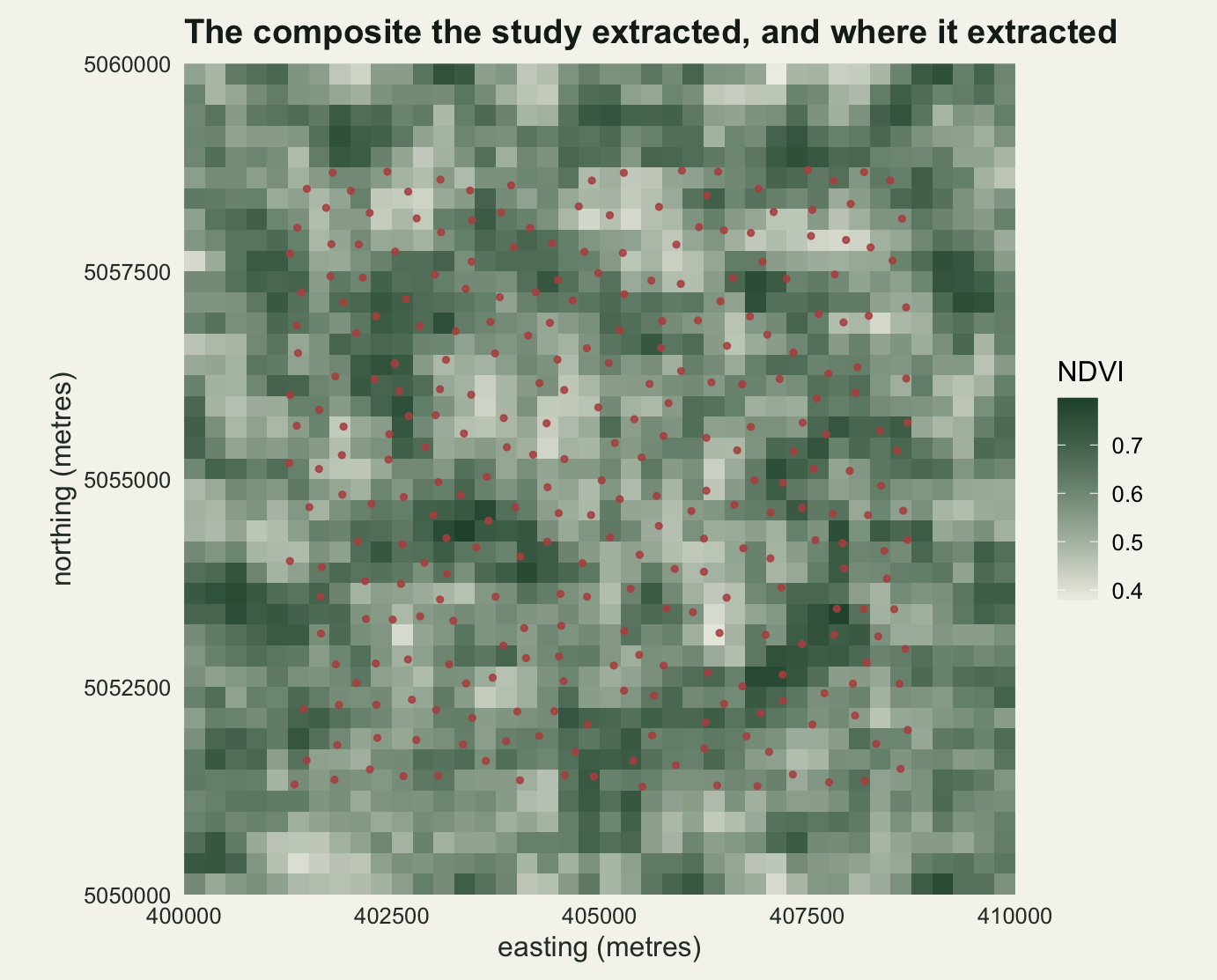
A shrub-steppe block of ten kilometres by ten kilometres, three hundred point count stations placed at random with a minimum separation of three hundred metres, and a scrub-nesting passerine counted as singing males over three visits in one breeding season. The habitat covariate is not measured in the field. It is downloaded: a growing-season mean NDVI composite at two hundred and fifty metre pixels, extracted at each station with one call to terra::extract, and put into a Poisson generalised linear model as the only predictor. The coefficient comes back positive, the p value has thirty-odd zeros in front of it, and the paper reports that abundance rises by more than a third for every tenth of an NDVI unit. Describing habitat over an area no field crew could walk is exactly what satellite data were brought into ecology to do (Kerr and Ostrovsky 2003), and the cost of it is that the predictor arrives from a pipeline nobody in the author list built.
That analysis has already happened. This post does not redo it and does not argue with the ecology. It takes the finished model and asks five questions about the covariate, in the order an auditor would ask them: is the raster on the grid the model thinks it is, does the extraction rule match the animal, is the grain right, was the image taken when the birds were counted, and does the model know that the covariate is an estimate rather than a measurement.
Three companion posts build the covariate itself and are not repeated here. NDVI time series from a raster stack assembles the cube. Harmonic regression on a seasonal raster fits the seasonal curve that a phenology metric comes from. Filling cloud gaps in a satellite series deals with the missing observations underneath both. Raster data in R with terra covers reading a layer, changing its grain and pulling values at points, so none of that mechanics is taught again below. What is new here is the arithmetic of what those choices do to an ecological coefficient.
Everything runs on simulated data, for the usual reason: a synthetic block comes with a truth column, so a coefficient can be scored rather than admired. True vegetation is generated at fifty metre subcells, the satellite product is a block average of it at two hundred and fifty metres with measurement error added, and the bird responds to the true vegetation averaged over a five hundred metre radius.
The study under test
The block holds two cover types in a mosaic: shrub patches and the grass matrix between them, and the bird nests in shrubs. Cover varies smoothly, so the fine grid holds a shrub fraction per subcell rather than a hard classification, and every NDVI value in the post is a mixture of the two cover types weighted by that fraction.
The six cover-type NDVI values below are the whole generating model. In mid-summer the shrubs are green and the grass has started to senesce, so NDVI rises with shrub cover. In April the order is reversed: the grass has flushed and the shrubs have not leafed out. In the previous, drier year the grass failed while the shrubs held on, so the mid-summer contrast between the cover types was wider than usual.
library(terra)

fine_res <- 50; fine_n <- 200          # true vegetation grid
pix <- 250; grid_n <- 40                # the satellite product
fct <- pix / fine_res
x0 <- 400000; y0 <- 5050000; win <- fine_n * fine_res

shift_torus <- function(M, dr, dc)
  M[((seq_len(nrow(M)) - 1 - dr) %% nrow(M)) + 1,
    ((seq_len(ncol(M)) - 1 - dc) %% ncol(M)) + 1]
box_smooth <- function(M, r) {
  out <- matrix(0, nrow(M), ncol(M))
  for (dr in -r:r) for (dc in -r:r) out <- out + shift_torus(M, dr, dc)
  out / (2 * r + 1)^2
}
disc_offsets <- function(r) {
  g <- expand.grid(dr = -r:r, dc = -r:r)
  as.matrix(g[g$dr^2 + g$dc^2 <= r^2, ])
}
disc_mean <- function(M, off) {
  out <- matrix(0, nrow(M), ncol(M))
  for (k in seq_len(nrow(off))) out <- out + shift_torus(M, off[k, 1], off[k, 2])
  out / nrow(off)
}
agg_mean <- function(M, f) {
  n <- nrow(M) / f
  a <- matrix(0, n, n)
  for (i in seq_len(f)) for (j in seq_len(f))
    a <- a + M[seq(i, by = f, length.out = n), seq(j, by = f, length.out = n)]
  a / f^2
}
as_layer <- function(A, cell) {
  r <- rast(xmin = x0, xmax = x0 + win, ymin = y0, ymax = y0 + win,
            resolution = cell, crs = "EPSG:32634")
  values(r) <- as.vector(t(A))
  names(r) <- "ndvi"
  r
}

set.seed(20260803)
zb <- box_smooth(matrix(rnorm(fine_n^2), fine_n, fine_n), 7)
zf <- box_smooth(matrix(rnorm(fine_n^2), fine_n, fine_n), 2)
zz <- 0.85 * zb / sd(as.vector(zb)) + 0.5 * zf / sd(as.vector(zf))
zz <- (zz - mean(zz)) / sd(as.vector(zz))
shrub_f <- plogis(1.15 * zz)

nd_sh_mid <- 0.78; nd_gr_mid <- 0.40
nd_sh_apr <- 0.52; nd_gr_apr <- 0.66
nd_sh_dry <- 0.72; nd_gr_dry <- 0.26
mix_ndvi <- function(sh, gr) gr + (sh - gr) * shrub_f
mid_f <- mix_ndvi(nd_sh_mid, nd_gr_mid)
apr_f <- mix_ndvi(nd_sh_apr, nd_gr_apr)
dry_f <- mix_ndvi(nd_sh_dry, nd_gr_dry)

home_r <- 500
ter_mid <- disc_mean(mid_f, disc_offsets(home_r / fine_res))

print(round(c(subcell_metres = fine_res, pixel_metres = pix,
              block_metres = win, home_range_radius = home_r,
              shrub_cover_mean = mean(shrub_f),
              july_contrast = nd_sh_mid - nd_gr_mid,
              april_contrast = nd_sh_apr - nd_gr_apr,
              drought_contrast = nd_sh_dry - nd_gr_dry), 4))
subcell_metres pixel_metres block_metres home_range_radius
50.0000 250.0000 10000.0000 500.0000
shrub_cover_mean july_contrast april_contrast drought_contrast
0.4992 0.3800 -0.1400 0.4600 The July contrast between pure shrub and pure grass is 0.38 NDVI units, the April contrast is -0.14, which is negative, and the drought-year contrast is 0.46. Hold those three numbers: check 4 is nothing but their ratios.
The response is the count of singing males at a station, Poisson around an expectation that depends on true July NDVI averaged over a 500 metre radius, the scale at which this species selects a territory. The true coefficient is set on that home-range average, and it is the only coefficient in the post that means anything on its own.
n_pt <- 300; edge_buf <- 1250; min_sep <- 300
set.seed(20260804)
px <- numeric(0); py <- numeric(0)
while (length(px) < n_pt) {
  cx <- runif(1, x0 + edge_buf, x0 + win - edge_buf)
  cy <- runif(1, y0 + edge_buf, y0 + win - edge_buf)
  if (length(px) == 0 || min((px - cx)^2 + (py - cy)^2) >= min_sep^2) {
    px <- c(px, cx); py <- c(py, cy)
  }
}
sub_j <- ceiling((px - x0) / fine_res)
sub_i <- ceiling((y0 + win - py) / fine_res)
x_true <- ter_mid[cbind(sub_i, sub_j)]

b_true <- 6; a0 <- log(8); xc <- mean(x_true)
mu_pt <- exp(a0 + b_true * (x_true - xc))
set.seed(20260805)
cnt <- rpois(n_pt, mu_pt)

true_per10 <- b_true / 10
true_per_sd <- b_true * sd(x_true)
print(round(c(stations = n_pt, mean_count = mean(cnt), max_count = max(cnt),
              empty_stations = sum(cnt == 0),
              sd_of_true_covariate = sd(x_true),
              true_coefficient_per_ndvi = b_true,
              true_coefficient_per_tenth = true_per10,
              true_effect_per_sd = true_per_sd), 4))
stations mean_count
300.0000 8.6400
max_count empty_stations
24.0000 1.0000
sd_of_true_covariate true_coefficient_per_ndvi
0.0455 6.0000
true_coefficient_per_tenth true_effect_per_sd
0.6000 0.2731 The survey returns a mean of 8.64 males per station, a maximum of 24, and 0.33 per cent of stations empty. The true coefficient is 6 per NDVI unit, or 0.6 per tenth of a unit, and the home-range average of true July NDVI has a standard deviation of 0.0455 across the stations, so the true effect per standard deviation of the covariate is 0.2731 on the log scale.
That last quantity does a lot of work below, so it is worth saying why. Every extraction rule and every grain in this post produces a different variable, and a coefficient per NDVI unit is a coefficient on whichever variable was extracted. Two of them are not comparable, because a value averaged over a kilometre has a smaller spread than a value read off one pixel and the same amount of ecology is divided by a smaller number. The effect per standard deviation of the covariate is comparable, and it has a true value.
The composite is the block average of true July NDVI over each two hundred and fifty metre pixel, plus measurement error in two parts: a smooth component standing for atmospheric correction residuals and view-angle effects, correlated over about a kilometre, and an independent per-pixel component standing for sensor noise and compositing. Both are added on the matrix before the layer is built, which avoids the trap that a bare numeric vector added to a SpatRaster recycles per layer rather than per cell.
sd_corr <- 0.025; sd_ind <- 0.015
mid_pix <- agg_mean(mid_f, fct)
make_err <- function(seed) {
  set.seed(seed)
  ec <- box_smooth(matrix(rnorm(grid_n^2), grid_n, grid_n), 2)
  ec / sd(as.vector(ec)) * sd_corr +
    matrix(rnorm(grid_n^2, 0, sd_ind), grid_n, grid_n)
}
err_mid <- make_err(20260806)
ndvi <- as_layer(mid_pix + err_mid, pix)
ndvi_clean <- as_layer(mid_pix, pix)
pv <- vect(cbind(px, py), type = "points", crs = crs(ndvi))
prc <- rowColFromCell(ndvi, cellFromXY(ndvi, cbind(px, py)))
err_sd <- sqrt(sd_corr^2 + sd_ind^2)
grid_gap <- max(abs(values(ndvi)[cellFromXY(ndvi, cbind(px, py))] -
                      (mid_pix + err_mid)[prc]))

print(c(layers = nlyr(ndvi), cells = ncell(ndvi)))
layers cells
1 1600 print(round(c(composite_error_sd = err_sd,
product_ndvi_min = min(values(ndvi)),
product_ndvi_max = max(values(ndvi)),
matrix_raster_gap = grid_gap), 5))composite_error_sd product_ndvi_min product_ndvi_max matrix_raster_gap
0.02915 0.37867 0.79707 0.00000 One layer of 1600 cells, a composite error standard deviation of 0.0292 NDVI units, and the largest disagreement between the matrix the truth was built in and the raster the analysis will read is 0.0. That last line is not decoration: building a raster from a matrix means committing to an ordering, and getting it wrong transposes the study area silently. The study itself is one extract and one glm.
fit_report <- function(w, y = cnt) {
  m <- glm(y ~ w, family = poisson)
  ci <- confint.default(m)
  c(b = unname(coef(m)[2]), se = unname(summary(m)$coefficients[2, 2]),
    lo = ci[2, 1], hi = ci[2, 2], p = unname(summary(m)$coefficients[2, 4]),
    aic = AIC(m), devx = 1 - m$deviance / m$null.deviance,
    per_sd = unname(coef(m)[2]) * sd(w))
}
nn <- extract(ndvi, pv, method = "simple")$ndvi
study <- fit_report(nn)
print(round(study[c("b", "se", "lo", "hi", "aic", "devx", "per_sd")], 4))
b se lo hi aic devx per_sd
3.2020 0.2622 2.6881 3.7159 1509.3898 0.3114 0.2422 print(round(c(per_tenth = study[["b"]] / 10,
lo_tenth = study[["lo"]] / 10, hi_tenth = study[["hi"]] / 10,
percent_per_tenth = 100 * (exp(study[["b"]] / 10) - 1),
sd_of_extracted = sd(nn)), 4)) per_tenth lo_tenth hi_tenth percent_per_tenth
0.3202 0.2688 0.3716 37.7405
sd_of_extracted
0.0756 The study reports 0.3202 per tenth of an NDVI unit, interval 0.2688 to 0.3716, a 37.74 per cent rise in abundance per tenth, with a p value of 2.7e-34 and 31.14 per cent of the deviance explained. Against a truth of 0.6 per tenth that is a little over half, but the two coefficients are on different variables, so the fair comparison is the standardised one: 0.2422 reported against 0.2731 true, a shortfall of 11.31 per cent. That is the number the five checks have to account for.
Check 1: is the covariate on the grid the model thinks it is
Two things can be wrong with the geometry and only one of them is visible. The first is a coordinate reference system mismatch, which is loud: the points land in the sea or in another hemisphere and the extraction returns nothing. The second is a small registration offset with everything else correct, which is silent.
Start with the loud one, because it takes two lines and it is the only geometric error a default workflow catches for free. Suppose the station coordinates were recorded in degrees and pasted into a projected file without transformation.
pv_bad <- vect(cbind(23.5 + (px - x0) / 1e5, 45.6 + (py - y0) / 1e5),
               type = "points", crs = crs(ndvi))
n_good <- sum(!is.na(extract(ndvi, pv, method = "simple")[, 2]))
n_bad <- sum(!is.na(extract(ndvi, pv_bad, method = "simple")[, 2]))
print(c(crs_strings_match = identical(crs(ndvi), crs(pv))))
crs_strings_match
TRUE print(c(good_points_returning_a_value = n_good,
bad_points_returning_a_value = n_bad))good_points_returning_a_value bad_points_returning_a_value
300 0 ext_tab <- rbind(raster = as.vector(ext(ndvi)), points = as.vector(ext(pv)),
degrees_pasted_in = as.vector(ext(pv_bad)))
print(round(ext_tab, 2)) xmin xmax ymin ymax
raster 400000.00 410000.00 5050000.00 5060000.00
points 401264.79 408705.90 5051298.63 5058718.54
degrees_pasted_in 23.51 23.59 45.61 45.69The comparison of extents is the whole diagnostic. The raster runs from 400000 to 410000 in the x direction; the honest points sit inside it and all 300 of them return a value; the degree-valued points sit at an x of about 23.5 and 0 of them return anything at all. Comparing crs() alone would not have caught it, because the broken object carries the correct projection string attached to the wrong numbers.
Now the silent one. Nothing above changes if the coordinates are right to within a pixel or two, and that is the case worth measuring: a shift from a datum realisation nobody recorded, a scanned map digitised against the wrong control points, or an uncorrected handheld fix under canopy. Sensor geolocation is rarely the culprit; Storey, Choate and Lee (2014) report Landsat 8 geolocation accuracy well inside a single pixel. The offsets that bite come from the biological coordinates, which is the case Velasquez-Tibata, Graham and Munch (2015) treat as a measurement error problem in species distribution models rather than as a data-cleaning one.
ang <- pi / 6
off_grid <- c(0, 0.2, 0.5, 1, 2)
off_tab <- t(sapply(off_grid, function(f) {
  qv <- vect(cbind(px + f * pix * cos(ang), py + f * pix * sin(ang)),
             type = "points", crs = crs(ndvi))
  v <- extract(ndvi, qv, method = "simple")[, 2]
  c(offset_pixels = f, offset_metres = f * pix, fit_report(v))
}))
off_tab <- as.data.frame(off_tab)
off_tab$lost_pct <- 100 * (1 - off_tab$b / off_tab$b[1])
print(round(off_tab[, c("offset_metres", "b", "se", "lo", "hi",
                        "devx", "per_sd", "lost_pct")], 4))
offset_metres b se lo hi devx per_sd lost_pct
1 0 3.2020 0.2622 2.6881 3.7159 0.3114 0.2422 0.0000
2 50 2.9141 0.2540 2.4162 3.4120 0.2735 0.2261 8.9912
3 125 2.7868 0.2662 2.2649 3.3086 0.2263 0.2045 12.9681
4 250 2.3419 0.2458 1.8602 2.8235 0.1870 0.1850 26.8629
5 500 1.5554 0.2530 1.0594 2.0513 0.0778 0.1196 51.4253print(round(c(se_ratio_two_pixels = off_tab$se[5] / off_tab$se[1],
interval_width_ratio =
(off_tab$hi[5] - off_tab$lo[5]) / (off_tab$hi[1] - off_tab$lo[1])), 4)) se_ratio_two_pixels interval_width_ratio
0.965 0.965 A fifth of a pixel, 50 metres, costs 8.99 per cent of the coefficient; one pixel costs 26.86 per cent and two pixels cost 51.43 per cent, taking the estimate from 3.202 down to 1.5554. The standard error does not follow. At two pixels of offset it is 0.253 against 0.2622, a ratio of 0.965, so the interval is 0.965 times as wide as the correctly registered one: the estimate halves and the reported precision improves slightly. Deviance explained does fall, from 31.14 to 7.78 per cent, but a single model has no second value to compare its fit against, so on its own that number says nothing.
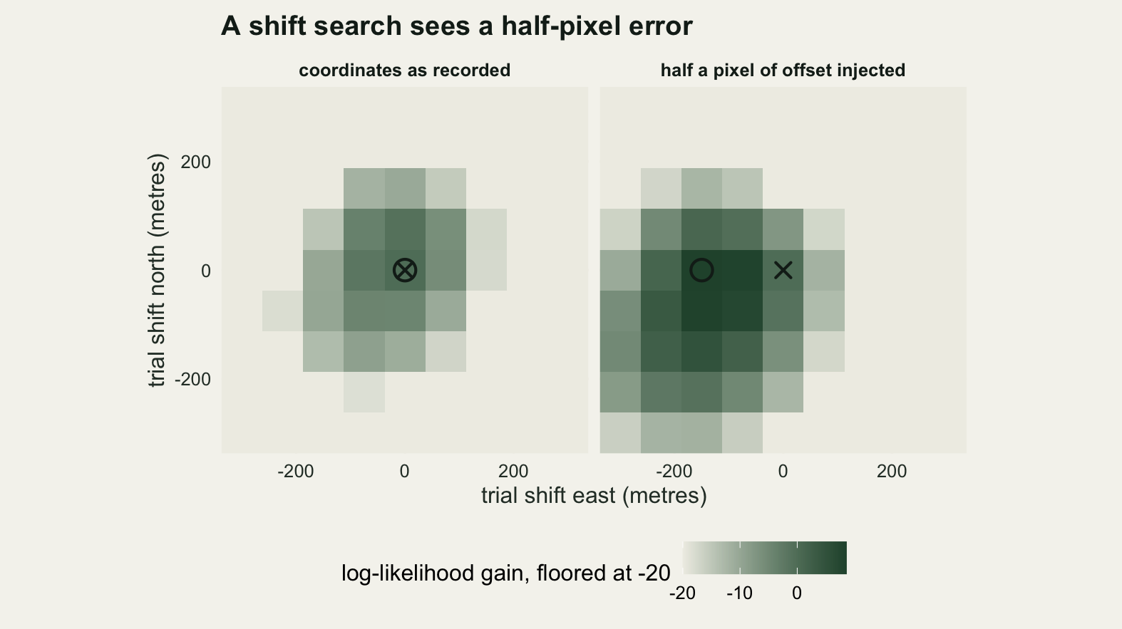
One diagnostic does see a shift, and it costs nothing. Slide the whole point set over a grid of candidate offsets, refit at each, and look at where the log-likelihood peaks; if the coordinates and the raster are registered to each other the peak should sit at zero. The search uses bilinear extraction, so the surface responds smoothly to a shift smaller than a pixel instead of stepping between cells.
sh_step <- 75
sh_gr <- expand.grid(dx = seq(-300, 300, by = sh_step),
                     dy = seq(-300, 300, by = sh_step))
cov_shift <- function(dx0, dy0)
  vapply(seq_len(nrow(sh_gr)), function(k) {
    qv <- vect(cbind(px + dx0 + sh_gr$dx[k], py + dy0 + sh_gr$dy[k]),
               type = "points", crs = crs(ndvi))
    extract(ndvi, qv, method = "bilinear")[, 2]
  }, numeric(n_pt))
ll_of <- function(y, Cm) apply(Cm, 2, function(v)
  as.numeric(logLik(glm(y ~ v, family = poisson))))

cs_true <- cov_shift(0, 0)
i00 <- which(sh_gr$dx == 0 & sh_gr$dy == 0)
ll_study <- ll_of(cnt, cs_true)
j_study <- which.max(ll_study)

dx_i <- 0.5 * pix * cos(ang); dy_i <- 0.5 * pix * sin(ang)
cs_off <- cov_shift(dx_i, dy_i)
ll_off <- ll_of(cnt, cs_off)
j_off <- which.max(ll_off)

print(round(c(candidate_offsets = nrow(sh_gr), step_metres = sh_step,
              study_best_dx = sh_gr$dx[j_study], study_best_dy = sh_gr$dy[j_study],
              study_gain = ll_study[j_study] - ll_study[i00]), 4))
candidate_offsets step_metres study_best_dx study_best_dy
81 75 0 0
study_gain
0 print(round(c(injected_dx = dx_i, injected_dy = dy_i,
recovered_dx = -sh_gr$dx[j_off], recovered_dy = -sh_gr$dy[j_off],
location_error = sqrt((sh_gr$dx[j_off] + dx_i)^2 +
(sh_gr$dy[j_off] + dy_i)^2),
injected_gain = ll_off[j_off] - ll_off[i00]), 4)) injected_dx injected_dy recovered_dx recovered_dy location_error
108.2532 62.5000 150.0000 0.0000 75.1601
injected_gain
8.6127 On the study as it stands the peak is at 0 metres east and 0 metres north, with a log-likelihood gain over the unshifted fit of 0.0000. On the same counts with a half-pixel offset injected, the search recovers 150 and 0 metres against an injected 108.3 and 62.5, missing by 75.16 metres, one step of the search grid, and gains 8.6127 in log-likelihood.
A maximum over 81 candidates is always positive, so the gain needs a reference distribution before it means anything. Simulating counts from the same expectation and rerunning the search supplies one.
n_null <- 100
set.seed(20260809)
gain_null <- dist_null <- numeric(n_null)
for (i in seq_len(n_null)) {
  lv <- ll_of(rpois(n_pt, mu_pt), cs_true)
  jj <- which.max(lv)
  gain_null[i] <- lv[jj] - lv[i00]
  dist_null[i] <- sqrt(sh_gr$dx[jj]^2 + sh_gr$dy[jj]^2)
}
q_gain <- unname(quantile(gain_null, c(0.5, 0.95)))
print(round(c(null_replicates = n_null, median_gain = q_gain[1],
              upper_5_percent_gain = q_gain[2],
              median_apparent_shift = median(dist_null),
              share_finding_zero = mean(dist_null == 0)), 4))
null_replicates median_gain upper_5_percent_gain
100.0000 1.7359 6.0930
median_apparent_shift share_finding_zero
75.0000 0.1800 print(round(c(study_gain = ll_study[j_study] - ll_study[i00],
study_percentile = mean(gain_null < ll_study[j_study] - ll_study[i00]),
injected_gain = ll_off[j_off] - ll_off[i00],
injected_percentile = mean(gain_null < ll_off[j_off] - ll_off[i00])), 4)) study_gain study_percentile injected_gain injected_percentile
0.0000 0.0000 8.6127 0.9900 On correctly registered data the search still finds something. The median gain over 100 null replicates is 1.7359, the median apparent shift is 75 metres, and the search lands exactly on zero in only 18 per cent of them. Against that distribution the injected half-pixel offset sits at the 99th percentile, so a shift of 125 metres is detectable; the study itself sits at the 0th.
Verdict: the study passes. The reference systems agree, every station returns a value, the map shows the points inside the grid, and the shift search returns the unshifted position with no likelihood gain at all, which is a better result than most correctly registered datasets give. The check also prices the failure it did not find: an undetected one-pixel offset would have removed 26.86 per cent of the coefficient while leaving the confidence interval the width it is now.
Check 2: does the extraction rule match the ecology
terra::extract with its defaults returns the value of the pixel the point falls in. That is a choice and it is an ecological one: it says the bird responds to the vegetation in the two hundred and fifty metre square it happens to be standing in and to nothing on the other side of the pixel boundary. Four other rules are equally defensible: bilinear interpolation between the four nearest pixel centres, and the mean over a buffer at each of three radii. The buffer means are computed twice, once with terra and once with a weight matrix built from the cell centres, because the fast version is needed again in check 5 and the two should agree to the last digit.
bl <- extract(ndvi, pv, method = "bilinear")$ndvi
buf_w <- function(r, radius) {
  xy <- xyFromCell(r, seq_len(ncell(r)))
  W <- matrix(0, n_pt, ncell(r))
  for (i in seq_len(n_pt)) {
    k <- (xy[, 1] - px[i])^2 + (xy[, 2] - py[i])^2 <= radius^2
    W[i, k] <- 1 / sum(k)
  }
  W
}
w500 <- buf_w(ndvi, 500)
buf_at <- function(radius) as.vector(buf_w(ndvi, radius) %*% values(ndvi)[, 1])
b250 <- buf_at(250)
b500 <- as.vector(w500 %*% values(ndvi)[, 1])
b1000 <- buf_at(1000)
terra_500 <- extract(ndvi, buffer(pv, width = 500, quadsegs = 60), fun = mean)$ndvi
print(c(terra_versus_weights = max(abs(terra_500 - b500)),
        cells_in_the_500_metre_buffer = median(rowSums(w500 > 0))))
terra_versus_weights cells_in_the_500_metre_buffer
2.220446e-16 1.300000e+01 rule_lab <- c("nearest pixel", "bilinear", "mean, 250 m", "mean, 500 m",
"mean, 1000 m")
rule_cov <- list(nn, bl, b250, b500, b1000)
rules <- as.data.frame(t(sapply(rule_cov, function(v)
c(sd_covariate = sd(v), cor_with_truth = cor(v, x_true), fit_report(v)))))
rules$rule <- rule_lab
rules$per_sd_pct_of_truth <- 100 * rules$per_sd / true_per_sd
print(cbind(rule = rule_lab,
round(rules[, c("sd_covariate", "cor_with_truth", "b", "se",
"lo", "hi", "per_sd", "devx",
"per_sd_pct_of_truth")], 4))) rule sd_covariate cor_with_truth b se lo hi per_sd
1 nearest pixel 0.0756 0.7239 3.2020 0.2622 2.6881 3.7159 0.2422
2 bilinear 0.0662 0.8015 3.8953 0.2984 3.3105 4.4801 0.2580
3 mean, 250 m 0.0626 0.8104 4.1592 0.3144 3.5430 4.7754 0.2602
4 mean, 500 m 0.0472 0.8863 5.7285 0.4146 4.9160 6.5411 0.2704
5 mean, 1000 m 0.0254 0.6846 8.2750 0.7918 6.7232 9.8268 0.2101
devx per_sd_pct_of_truth
1 0.3114 88.6916
2 0.3550 94.4740
3 0.3633 95.2879
4 0.3951 99.0021
5 0.2301 76.9263print(round(c(spread_in_coefficient = max(rules$b) / min(rules$b),
spread_in_per_sd = max(rules$per_sd) / min(rules$per_sd),
best_matched_rule_per_sd = rules$per_sd[4],
true_per_sd = true_per_sd), 4)) spread_in_coefficient spread_in_per_sd best_matched_rule_per_sd
2.5843 1.2870 0.2704
true_per_sd
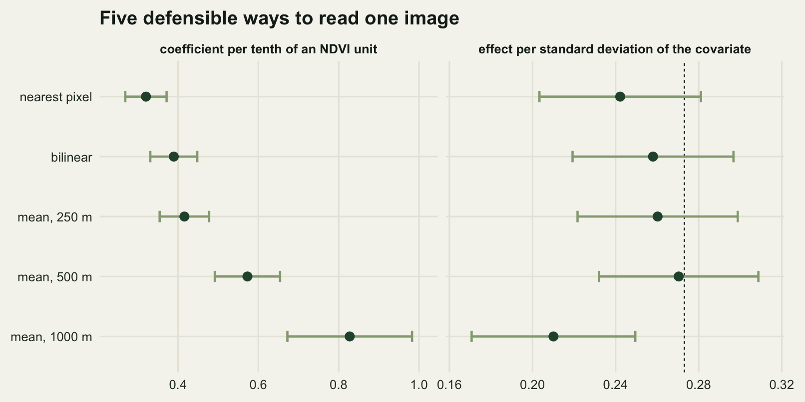
0.2731 The five rules give coefficients from 3.202 to 8.275 per NDVI unit, a factor of 2.5843. Read as the paper would read it, the same birds and the same image support anything from 37.74 to 128.76 per cent more birds per tenth of an NDVI unit. Deviance explained runs from 23.01 to 39.51 per cent, which does order the rules, but the differences are small next to the differences in the estimate.
Most of that spread is units rather than ecology. The standard deviation of the extracted covariate falls from 0.0756 at the nearest pixel to 0.0254 at the kilometre buffer, because averaging over a wider area removes variation. Divide it out and the effect per standard deviation runs from 0.2101 to 0.2704, a factor of 1.287 instead of 2.5843. Gotway and Young (2002) set out the general form: a covariate averaged over one spatial support and a response measured on another are different variables, and the coefficient linking them is a property of the pair rather than of the ecology.
What is left is ecology, and here it can be scored against a true effect per standard deviation of 0.2731. The five rules recover 88.69, 94.47, 95.29, 99 and 76.93 per cent of it. The winner is the five hundred metre buffer, the radius the bird integrates over, which lands within 1 per cent of the truth. The default nearest pixel loses 11.31 per cent and the kilometre buffer, averaging over four times the area the bird uses, loses 23.07 per cent.
Verdict: the study made an ecological hypothesis without stating it. The default rule is not wrong in any sense a referee could point at, and it is not the rule this species implies. The correlation with the truth is the mechanism: 0.7239 at the nearest pixel against 0.8863 at the matched buffer. The recommendation is not to use buffers. It is that the radius is a parameter of the ecology, that it should be argued for in the methods, and that the spread across defensible radii belongs next to the confidence interval. On the standardised scale, where the five rules are comparable, that spread is 0.78 times the width of the interval. The choice of radius costs less than the sampling error does, and unlike the sampling error it is never reported.
Check 3: is the grain right, and what does coarsening do
The same product usually exists at several resolutions, and the coarser one is smaller to download, faster to reproject and often the only one with a long archive. Aggregating the composite and refitting says what that costs. The extraction rule is held at the study’s nearest pixel throughout, so the only thing changing is the size of the pixel.
grain_fac <- c(1, 2, 4, 8)
grain <- as.data.frame(t(sapply(grain_fac, function(f) {
  rg <- if (f == 1) ndvi else aggregate(ndvi, fact = f, fun = "mean")
  rc <- if (f == 1) ndvi_clean else aggregate(ndvi_clean, fact = f, fun = "mean")
  v <- extract(rg, pv, method = "simple")[, 2]
  vc <- extract(rc, pv, method = "simple")[, 2]
  fc <- fit_report(vc)
  c(cell_metres = res(rg)[1], cells = ncell(rg), sd_covariate = sd(v),
    cor_with_truth = cor(v, x_true), fit_report(v),
    b_without_composite_error = fc[["b"]])
})))
grain$per_sd_pct_of_truth <- 100 * grain$per_sd / true_per_sd
print(round(grain[, c("cell_metres", "cells", "sd_covariate", "cor_with_truth",
                      "b", "se", "lo", "hi")], 4))
cell_metres cells sd_covariate cor_with_truth b se lo hi
1 250 1600 0.0756 0.7239 3.2020 0.2622 2.6881 3.7159
2 500 400 0.0614 0.7736 4.0368 0.3241 3.4016 4.6720
3 1000 100 0.0428 0.6580 4.3561 0.4572 3.4599 5.2523
4 2000 25 0.0217 0.4279 6.0135 0.9169 4.2163 7.8106print(round(grain[, c("cell_metres", "per_sd", "per_sd_pct_of_truth", "devx",
"aic", "b_without_composite_error")], 4)) cell_metres per_sd per_sd_pct_of_truth devx aic
1 250 0.2422 88.6916 0.3114 1509.390
2 500 0.2479 90.7594 0.3248 1502.951
3 1000 0.1865 68.2718 0.1878 1569.042
4 2000 0.1305 47.7751 0.0899 1616.281
b_without_composite_error
1 3.6261
2 4.2524
3 4.8326
4 5.5471print(round(c(coefficient_ratio = grain$b[4] / grain$b[1],
se_ratio = grain$se[4] / grain$se[1],
per_sd_ratio = grain$per_sd[4] / grain$per_sd[1],
deviance_ratio = grain$devx[4] / grain$devx[1]), 4))coefficient_ratio se_ratio per_sd_ratio deviance_ratio
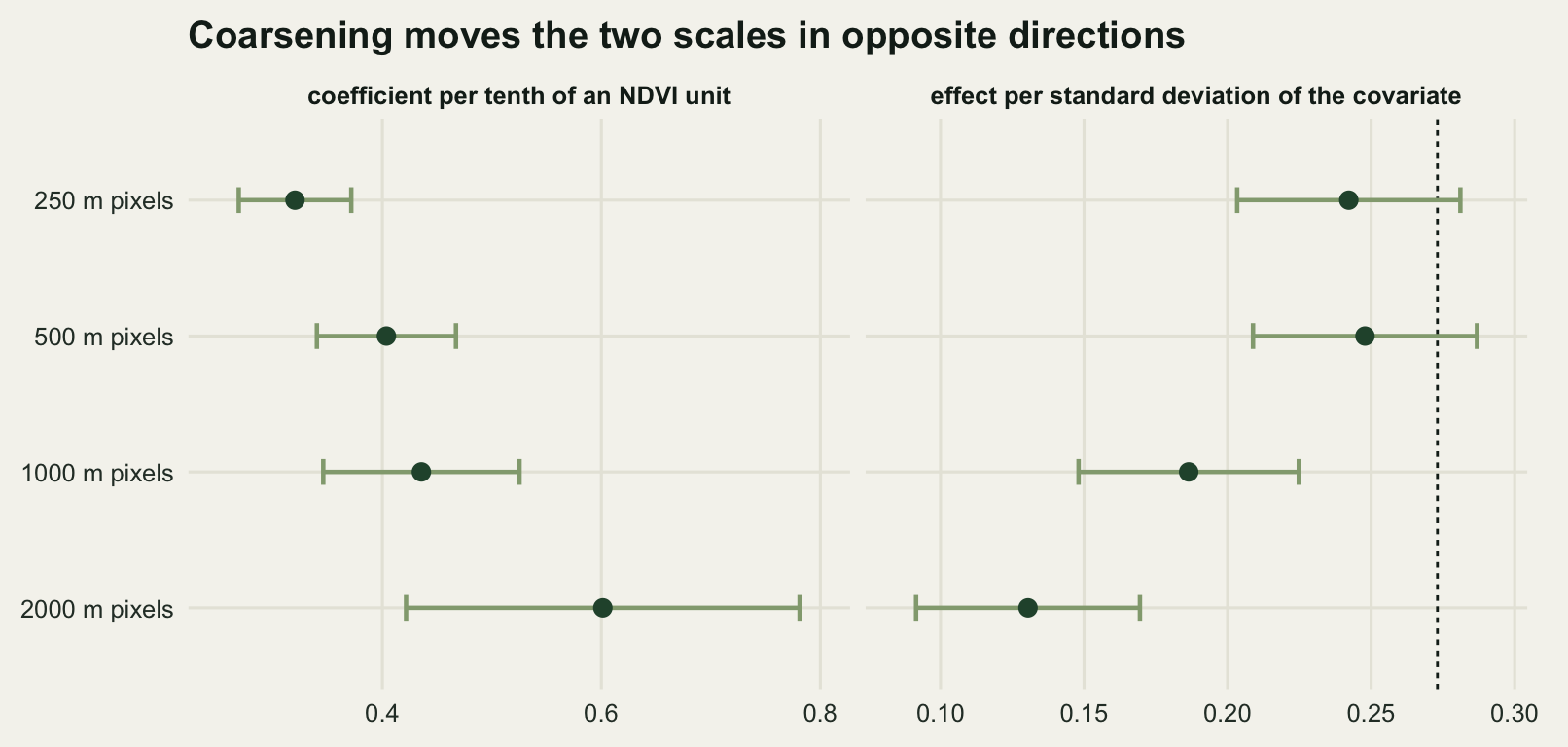
1.8780 3.4970 0.5387 0.2886 The coefficient per NDVI unit rises with the pixel: 3.202 at 250 metres, 4.0368 at 500, 4.3561 at 1000 and 6.0135 at 2000, a factor of 1.878 across the range. Taken at face value that reads as a stronger relationship at coarse grain, which is the opposite of what is happening.
Three other columns say what is happening. The standard deviation of the covariate falls from 0.0756 to 0.0217, so the same response is divided by a bit over a quarter of the spread. The correlation with the truth falls from 0.7239 to 0.4279. And the comparable quantity, the effect per standard deviation, falls from 0.2422 to 0.1305, which is 88.69 per cent of the truth at the native grain and 47.78 per cent at two kilometres. Deviance explained falls from 31.14 to 8.99 per cent and AIC rises by 106.89.
This check was set up to test a specific prediction and the prediction did not come out. It was that coarsening would give a confident, shrunken effect: an attenuated coefficient with a standard error that fails to grow to match. The attenuation is real, 46.13 per cent on the standardised scale, but the standard error grows by a factor of 3.497, which is more than enough, and the interval at two kilometre pixels is wide and honest rather than narrow and wrong. Coarsening degrades a covariate in a way that shows up in every fit statistic on the printout. The confident, shrunken estimate is what check 1 produced, where the coefficient halved and the interval did not move at all.
One column separates the two things coarsening does at once. Aggregating averages the composite error away as well as the signal, so a coarse covariate is less noisy and more mismatched at the same time.
gs <- data.frame(cell_metres = grain$cell_metres,
                 with_error = grain$b, without_error = grain$b_without_composite_error)
gs$error_share_pct <- 100 * (1 - gs$with_error / gs$without_error)
print(round(gs, 4))
cell_metres with_error without_error error_share_pct
1 250 3.2020 3.6261 11.6945
2 500 4.0368 4.2524 5.0693
3 1000 4.3561 4.8326 9.8606
4 2000 6.0135 5.5471 -8.4076At the native grain the composite error pulls the coefficient down by 11.69 per cent relative to the same analysis on an error-free product. By two kilometre pixels that penalty is -8.41 per cent, which is negative: the error has been averaged away so thoroughly that what is left is swamped. The mismatch penalty has grown throughout. The sequence in between is not monotone, partly because each grain sees one realisation of the error field, and that is the practical reason a grain cannot be chosen by watching the coefficient.
Verdict: the study used the finest grain available, and the printout could not have told it whether that was the right call. At the native grain the standardised effect is 88.69 per cent of the truth, one step of coarsening to 500 metre pixels scores slightly better at 90.76 per cent, and the coarsest grain tested keeps 47.78 per cent. The case for the finest grain rests on what happens from 1000 metres onwards rather than on 250 metres being the best row. Anyone reading the coefficient alone would conclude the opposite, reading a change in units as a change in biology.
Check 4: was the covariate measured when the birds were counted
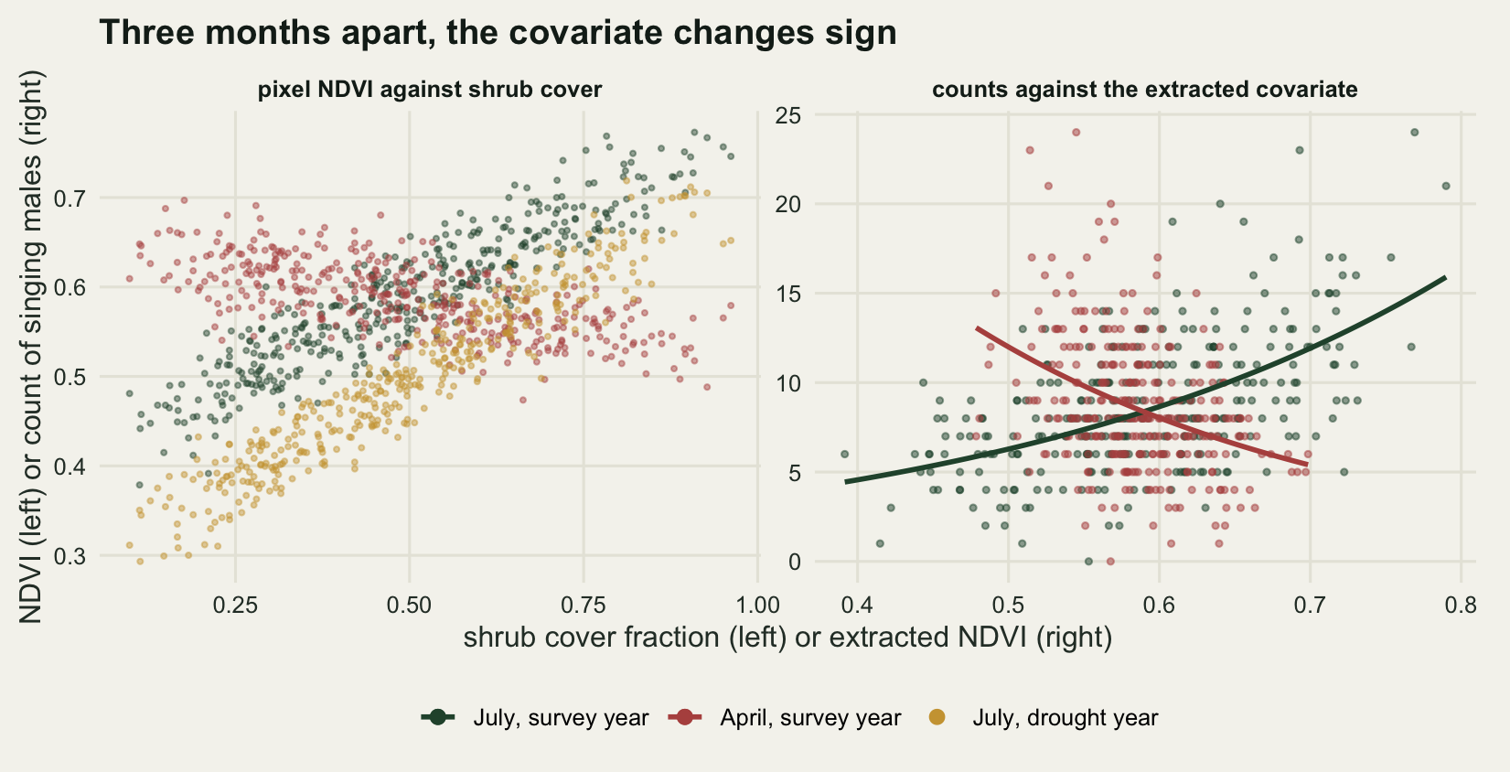
A growing-season composite has a window and somebody chose it. The three images built at the top of the post are the same block under three windows: the July composite that matches the survey, an April composite from the same year, and a July composite from the previous, drier year. All three are legitimate products and all three would be described in a methods section as growing-season NDVI.
r_apr <- as_layer(agg_mean(apr_f, fct) + make_err(20260807), pix)
r_dry <- as_layer(agg_mean(dry_f, fct) + make_err(20260808), pix)
apr_pt <- extract(r_apr, pv, method = "simple")$ndvi
dry_pt <- extract(r_dry, pv, method = "simple")$ndvi
season_lab <- c("July, survey year", "April, survey year", "July, drought year")
season <- as.data.frame(t(sapply(list(nn, apr_pt, dry_pt), fit_report)))
season$image <- season_lab
season$per_sd_pct_of_truth <- 100 * season$per_sd / true_per_sd
contrast_ratio <- (nd_sh_dry - nd_gr_dry) / (nd_sh_mid - nd_gr_mid)
season$sd_covariate <- c(sd(nn), sd(apr_pt), sd(dry_pt))
season$predicted_b <- study[["b"]] * (nd_sh_mid - nd_gr_mid) /
  c(nd_sh_mid - nd_gr_mid, nd_sh_apr - nd_gr_apr, nd_sh_dry - nd_gr_dry)
print(cbind(image = season_lab,
            round(season[, c("sd_covariate", "b", "se", "lo", "hi", "devx",
                             "per_sd", "per_sd_pct_of_truth", "predicted_b")], 4)))
image sd_covariate b se lo hi devx per_sd
1 July, survey year 0.0756 3.2020 0.2622 2.6881 3.7159 0.3114 0.2422
2 April, survey year 0.0408 -4.0112 0.4883 -4.9683 -3.0542 0.1411 -0.1637
3 July, drought year 0.0888 2.6944 0.2276 2.2484 3.1404 0.2964 0.2392
per_sd_pct_of_truth predicted_b
1 88.6916 3.2020
2 -59.9565 -8.6912
3 87.5789 2.6451print(round(c(drought_over_july_contrast = contrast_ratio,
drought_coefficient = season$b[3],
drought_predicted = season$predicted_b[3],
deviance_july = season$devx[1],
deviance_drought = season$devx[3]), 4))drought_over_july_contrast drought_coefficient
1.2105 2.6944
drought_predicted deviance_july
2.6451 0.3114
deviance_drought
0.2964 The drought-year image is the dangerous one. It ranks the pixels in the same order as the July image, because shrub cover has not changed, so nothing about the fit looks unusual: deviance explained is 29.64 per cent against 31.14 per cent for the matched image, and the coefficient is significant at any threshold. But the contrast between the cover types was 1.2105 times wider in the drought year, so the same ecology is spread over a wider NDVI axis and the coefficient shrinks by that factor. Rescaling the matched coefficient by the ratio of contrasts predicts 2.6451, and the fitted value is 2.6944, agreeing to 1.86 per cent. A reader comparing that coefficient with one from a wetter year is comparing two different rulers.
The April image is the loud failure. Its coefficient is -4.0112 per NDVI unit, negative, with an interval from -4.9683 to -3.0542 and 14.11 per cent of the deviance explained. A study using it would report with high confidence that this bird avoids green vegetation, and nothing in the model output would be wrong. In April the grass is the green thing and the shrubs are not, so the covariate has changed sign relative to the habitat while keeping its name. The same rescaling that worked for the drought year predicts -8.6912 here and the fit returns only -4.0112, because the April image spreads the same shrub gradient over a standard deviation of 0.0408 against 0.0756 in July, so the same composite error attenuates it much harder. Pettorelli and colleagues (2005) make the general point that NDVI tracks the phenology of whatever is dominant at the moment of the image; check 4 is what that costs when the moment is wrong by three months.
The mixed-pixel version of the problem lives inside a single image. A pixel that straddles shrub and grass returns a value describing neither. Splitting the stations by how heterogeneous their own pixel is, measured as the standard deviation of true NDVI among the twenty-five subcells inside it, puts a number on it.
het_pix <- sqrt(pmax(agg_mean(mid_f^2, fct) - mid_pix^2, 0))
het_pt <- het_pix[prc]
mixed_half <- het_pt > median(het_pt)
mixed <- as.data.frame(rbind(
  homogeneous = fit_report(nn[!mixed_half], cnt[!mixed_half]),
  mixed = fit_report(nn[mixed_half], cnt[mixed_half])))
mixed$stations <- c(sum(!mixed_half), sum(mixed_half))
mixed$within_pixel_sd <- c(mean(het_pt[!mixed_half]), mean(het_pt[mixed_half]))
print(round(mixed[, c("stations", "within_pixel_sd", "b", "se", "lo", "hi",
                      "devx", "per_sd")], 4))
stations within_pixel_sd b se lo hi devx per_sd
homogeneous 150 0.0339 3.3020 0.3134 2.6878 3.9162 0.4025 0.2962
mixed 150 0.0581 2.9173 0.4752 1.9860 3.8486 0.1873 0.1705print(round(c(coefficient_gap = mixed$b[1] - mixed$b[2],
gap_se = sqrt(mixed$se[1]^2 + mixed$se[2]^2),
deviance_ratio = mixed$devx[1] / mixed$devx[2]), 4))coefficient_gap gap_se deviance_ratio
0.3847 0.5692 2.1488 The homogeneous half has a mean within-pixel standard deviation of 0.0339 NDVI units and the mixed half 0.0581. Their coefficients are 3.302 and 2.9173, a gap of 0.3847 against a standard error on the gap of 0.5692, so on 300 stations the two coefficients are not distinguishable. What is distinguishable is the fit: the homogeneous half explains 40.25 per cent of its deviance and the mixed half 18.73 per cent, a ratio of 2.1488. Half the stations carry most of the signal.
Verdict: the study passes on timing and is exposed on comparability. The composite window does match the survey, which is the part that matters most and the part the April fit shows would have been fatal. What the study cannot do is set its coefficient beside one from another year or another sensor, because the number carries the contrast of its own image in its units.
Check 5: the covariate is an estimate and the model treats it as measured
The NDVI value in a pixel of a composite is not a measurement of that pixel. It is the output of an atmospheric correction, a cloud mask, a compositing rule and, if the covariate is a seasonal amplitude or a phenology date, a fitted harmonic model on top of all that. Foody (2002) is the standard argument that a remote sensing product arrives with an accuracy statement and that the statement belongs in the analysis; a GLM given the product as a predictor assumes the accuracy is perfect.
The estimand has to be stated carefully, because checks 2 and 3 established that every extraction produces its own variable. Holding the extraction at the study’s rule, the target is the coefficient the study would have obtained from an error-free version of the same product at the same pixels. The run below redraws the composite error and the counts three hundred times over the same block and the same stations, fits the naive model to the noisy covariate and the same model to the error-free one, and compares.
run_studies <- function(n_rep, sdc, sdi, seed0) {
  var_e <- sdc^2 + sdi^2
  out <- matrix(NA_real_, n_rep, 7)
  w_clean <- mid_pix[prc]
  for (i in seq_len(n_rep)) {
    set.seed(seed0 + i)
    ec <- box_smooth(matrix(rnorm(grid_n^2), grid_n, grid_n), 2)
    w <- (mid_pix + ec / sd(as.vector(ec)) * sdc +
            matrix(rnorm(grid_n^2, 0, sdi), grid_n, grid_n))[prc]
    y <- rpois(n_pt, mu_pt)
    m <- glm(y ~ w, family = poisson); mc <- glm(y ~ w_clean, family = poisson)
    bb <- unname(coef(m)[2]); ss <- unname(summary(m)$coefficients[2, 2])
    lam <- 1 - var_e / var(w)
    out[i, ] <- c(bb, ss, lam, bb / lam, ss / lam,
                  unname(coef(mc)[2]), unname(summary(mc)$coefficients[2, 2]))
  }
  colnames(out) <- c("b", "se", "lam", "b_rc", "se_rc", "b_cl", "se_cl")
  as.data.frame(out)
}
n_rep <- 300
run1 <- run_studies(n_rep, sd_corr, sd_ind, 771000)
b_ref <- mean(run1$b_cl)
cvg <- function(e, s) mean(abs(e - b_ref) < 1.96 * s)
err5 <- c(replicates = n_rep, target_coefficient = b_ref,
          mean_reliability = mean(run1$lam),
          naive_mean = mean(run1$b), naive_coverage = cvg(run1$b, run1$se),
          naive_width = mean(3.92 * run1$se),
          corrected_mean = mean(run1$b_rc),
          corrected_coverage = cvg(run1$b_rc, run1$se_rc),
          corrected_width = mean(3.92 * run1$se_rc),
          oracle_coverage = cvg(run1$b_cl, run1$se_cl))
print(round(err5, 4))
replicates target_coefficient mean_reliability naive_mean
300.0000 3.1834 0.8552 2.6988
naive_coverage naive_width corrected_mean corrected_coverage
0.5133 1.0442 3.1567 0.9300
corrected_width oracle_coverage
1.2216 0.9567 print(round(c(attenuation_pct = 100 * (1 - mean(run1$b) / b_ref),
predicted_attenuation_pct = 100 * (1 - mean(run1$lam)),
width_ratio = mean(run1$se_rc) / mean(run1$se),
bias_in_se_units = (b_ref - mean(run1$b)) / mean(run1$se)), 4)) attenuation_pct predicted_attenuation_pct width_ratio
15.2241 14.4839 1.1698
bias_in_se_units
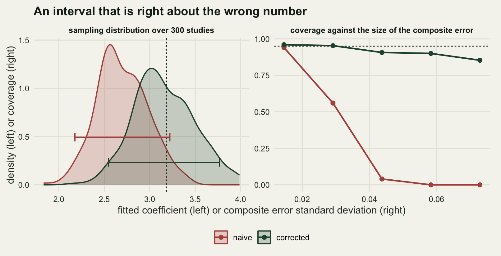
1.8193 Over 300 replicates the naive coefficient averages 2.6988 against a target of 3.1834, an attenuation of 15.22 per cent, which the reliability ratio predicts at 14.48 per cent. That is the ordinary regression dilution covered in measurement error and regression dilution, arriving by a route nobody files under measurement error.
The coverage is the finding. The naive ninety five per cent interval contains the target in 51.33 per cent of replicates against 95.67 per cent for the same model given the error-free covariate. The bias is 1.8193 standard errors, and a bias of that size against an interval of that width fails about half the time.
The repair is the oldest one in the measurement error toolkit. With the error variance known, replace the covariate by its conditional expectation given the observed value, which for classical additive error is the observed value shrunk towards its mean by the reliability ratio. For a single predictor that is an affine transformation, so the corrected coefficient and its standard error are both the naive ones divided by the reliability.
lam_grid <- c(0.85, 0.925, 1, 1.075, 1.15)
sens <- t(sapply(lam_grid, function(f) {
  l2 <- pmin(run1$lam * f, 0.999)
  c(reliability_used = mean(l2), multiplier = f,
    mean_estimate = mean(run1$b / l2), coverage = cvg(run1$b / l2, run1$se / l2))
}))
print(round(sens, 4))
reliability_used multiplier mean_estimate coverage
[1,] 0.7269 0.850 3.7138 0.6767
[2,] 0.7910 0.925 3.4127 0.8767
[3,] 0.8552 1.000 3.1567 0.9300
[4,] 0.9193 1.075 2.9365 0.8667
[5,] 0.9832 1.150 2.7456 0.6000print(round(c(true_reliability = mean(run1$lam),
corrected_mean = mean(run1$b_rc),
corrected_coverage = err5[["corrected_coverage"]],
precision_cost = err5[["corrected_width"]] / err5[["naive_width"]]), 4)) true_reliability corrected_mean corrected_coverage precision_cost
0.8552 3.1567 0.9300 1.1698 With the correct reliability the corrected estimate averages 3.1567 against the target 3.1834 and coverage returns to 93 per cent. The precision cost is exactly the reliability: the interval is 1.1698 times wider, which for a correction that moves the point estimate by 16.97 per cent is a cheap trade.
The sensitivity rows are the caveat, and it is the caveat checking a measurement-error correction reaches from the other side. Getting the reliability wrong by fifteen per cent in either direction drops coverage to 67.67 and 60 per cent: still better than the naive 51.33 per cent, but a long way short of nominal in both directions. The correction is only as good as the error variance behind it, and for a satellite product that number has to come from repeat scenes within the compositing window, an independent sensor over the same pixels, or the prediction standard error of the harmonic fit if the covariate is a fitted phenology metric. Stoklosa and colleagues (2015) work the same problem for climate surfaces in species distribution models and reach the same place, using simulation-extrapolation where the closed form runs out: that method is set out in correcting measurement error with SIMEX and follows Cook and Stefanski (1994).
How much this matters depends on how large the error is, and a covariate that has been through a harmonic fit or a gap filler carries more of it than a plain composite.
n_sweep <- 150
sweep_sc <- c(0.5, 1, 1.5, 2, 2.5)
err_sweep <- t(sapply(sweep_sc, function(s) {
  rs <- run_studies(n_sweep, sd_corr * s, sd_ind * s, 880000 + 1000 * s)
  tgt <- mean(rs$b_cl)
  c(error_sd = sqrt((sd_corr * s)^2 + (sd_ind * s)^2),
    reliability = mean(rs$lam), naive_b = mean(rs$b),
    naive_coverage = mean(abs(rs$b - tgt) < 1.96 * rs$se),
    corrected_b = mean(rs$b_rc),
    corrected_coverage = mean(abs(rs$b_rc - tgt) < 1.96 * rs$se_rc))
}))
err_sweep <- as.data.frame(err_sweep)
print(round(err_sweep, 4))
error_sd reliability naive_b naive_coverage corrected_b corrected_coverage
1 0.0146 0.9594 3.0185 0.94 3.1462 0.9600
2 0.0292 0.8552 2.6833 0.56 3.1380 0.9533
3 0.0437 0.7251 2.2865 0.04 3.1560 0.9067
4 0.0583 0.5955 1.8903 0.00 3.1839 0.9000
5 0.0729 0.4777 1.5090 0.00 3.1993 0.8533At a composite error standard deviation of 0.0146 NDVI units the naive interval still covers 94 per cent of the time. At 0.0437 it covers 4 per cent and at 0.0729 it covers 0 per cent, which is to say never. The corrected interval holds between 85.33 and 96 per cent across the range.
Verdict: the study fails this check and does not know it. Its covariate carries an error standard deviation of 0.0292 NDVI units, giving a reliability of 0.8552, an attenuation of 14.48 per cent and a reported interval that covers the right answer 51.33 per cent of the time. Nothing on the model summary indicates it, and the repair needs one number the study never obtained.
The honest limit
The five checks are not interchangeable. Check 1 catches a geometric error that leaves the interval untouched, and it passed here. Check 2 catches a silent ecological assumption and is the only one of the five that moves the coefficient by more than a factor of two with nothing done wrong anywhere. Check 3 catches a grain that has stopped resolving the animal, and it announces itself in every fit statistic. Check 4 catches an image from the wrong moment and is the only one that can change the sign. Check 5 catches an interval that is right about the wrong number and is the only one that needs information from outside the dataset.
Two of them are weak. The mixed-pixel split in check 4 could not distinguish the two coefficients at 300 stations, a gap of 0.3847 against a standard error of 0.5692, and the difference in deviance explained was the only usable signal. The shift search in check 1 finds an apparent offset of 75 metres on correctly registered data more often than not, so it needs a simulated null before any peak in it can be believed.
The larger limit is the one every simulation-based check on this blog shares. There is a truth column here, so each check ends in a verdict; on real data none of them does. The extraction sweep in check 2 returns a spread and no way to score it, the grain sweep in check 3 returns a sequence with no limit visible, and the reliability in check 5 has to be measured rather than looked up. What these checks buy in the field is the spread, and the spread is worth reporting precisely because it is usually wider than the confidence interval next to it.
Three classes of remote sensing error have no analogue in this post at all, and all three are larger in the field than anything simulated above. Atmospheric correction leaves residuals that are spatially and temporally structured rather than random, so they behave like a confounder rather than like noise. Sensors drift and are replaced, and cross-sensor calibration between generations of an instrument is a splice in the middle of a series of the kind splicing a monitoring series measures. Reflectance depends on the angles between the sun, the surface and the sensor, so two images of the same unchanged vegetation differ, and a composite averages over a set of geometries that varies across the scene. Above all, the product downloaded from an archive has already had somebody else’s model applied to it: a cloud mask, a bidirectional reflectance adjustment, a gap filler, sometimes a fitted phenology curve. Gottschalk, Huettmann and Ehlers (2005) reviewed three decades of bird habitat work built on satellite imagery and found the properties of the imagery reported far less often than the properties of the bird data, which is the same imbalance this post is about.
Three narrower limits belong on the record. The counts here are independent given the covariate, and stations three hundred metres apart in real shrub-steppe would not be, so every standard error in the post is optimistic. Detection probability is set to one, and a covariate that predicts detectability as well as abundance would add a bias none of these checks looks for. And the phenological reversal in check 4 was built into the generating model, so its magnitude demonstrates that a seasonal mismatch can reverse a sign rather than estimating how often it does.
Where to go next
The cheapest of these to run on an analysis you already have is check 2, and it takes ten minutes: extract the covariate again at two or three other radii, refit, and set the coefficients side by side on the standardised scale. If they move by more than the confidence interval, the paper’s single number is a choice rather than a result and the choice should be argued for. The second cheapest is the drought-year arithmetic in check 4, which needs no code: work out what contrast in the index the cover types produced in the image you used, and ask whether it was the same in the study you are comparing yourself with.
For the machinery underneath, raster data in R with terra covers extraction and aggregation, and NDVI time series from a raster stack builds the cube these composites come from. The measurement error cluster carries the corrections check 5 only touches: measurement error and regression dilution for the reliability ratio, correcting measurement error with SIMEX for the case where no closed form exists, and checking a measurement-error correction for where the reliability comes from. The standard errors here assume the stations are independent, which stations three hundred metres apart are not, and the tool for finding out how bad that is over a block like this one is spatial autocorrelation and Moran’s I.
References
Pettorelli N, Vik JO, Mysterud A, Gaillard JM, Tucker CJ, Stenseth NC 2005 Trends in Ecology and Evolution 20(9):503-510 (10.1016/j.tree.2005.05.011)
Kerr JT, Ostrovsky M 2003 Trends in Ecology and Evolution 18(6):299-305 (10.1016/S0169-5347(03)00071-5)
Gottschalk TK, Huettmann F, Ehlers M 2005 International Journal of Remote Sensing 26(12):2631-2656 (10.1080/01431160512331338041)
Foody GM 2002 Remote Sensing of Environment 80(1):185-201 (10.1016/S0034-4257(01)00295-4)
Storey J, Choate M, Lee K 2014 Remote Sensing 6(11):11127-11152 (10.3390/rs61111127)
Gotway CA, Young LJ 2002 Journal of the American Statistical Association 97(458):632-648 (10.1198/016214502760047140)
Velasquez-Tibata J, Graham CH, Munch SB 2015 Ecography 39(3):305-316 (10.1111/ecog.01205)
Stoklosa J, Daly C, Foster SD, Ashcroft MB, Warton DI 2015 Methods in Ecology and Evolution 6(4):412-423 (10.1111/2041-210X.12217)
Cook JR, Stefanski LA 1994 Journal of the American Statistical Association 89(428):1314-1328 (10.1080/01621459.1994.10476871)