library(ggplot2)
library(patchwork)
library(sf)

te_paper  <- "#f5f4ee"
te_ink    <- "#16241d"
te_body   <- "#2c3a31"
te_forest <- "#275139"
te_rust   <- "#b5534e"
te_gold   <- "#c9b458"
te_line   <- "#dad9ca"

theme_datasheet <- function() {
  theme_minimal(base_size = 12) +
    theme(plot.background  = element_rect(fill = te_paper, colour = NA),
          panel.background = element_rect(fill = te_paper, colour = NA),
          panel.grid.major = element_line(colour = te_line, linewidth = 0.3),
          panel.grid.minor = element_blank(),
          text             = element_text(colour = te_body),
          plot.title       = element_text(colour = te_ink, face = "bold"),
          plot.subtitle    = element_text(colour = te_body),
          axis.text        = element_text(colour = te_body))
}

utm <- "EPSG:32634"; x_org <- 400000; y_org <- 5050000; ext_m <- 5000
hab_frac <- 0.2
a_ext <- ext_m^2; a_hab <- hab_frac * a_ext; a_mat <- a_ext - a_hab
lg_avail <- log(a_hab / a_mat)
k_geom <- sqrt(2 / pi)

box_of <- function(a, b, wd, ht)
  st_polygon(list(cbind(c(a, a + wd, a + wd, a, a), c(b, b, b + ht, b + ht, b))))
blk <- st_sfc(box_of(x_org, y_org, ext_m, ext_m), crs = utm)
as_pts <- function(m)
  st_as_sf(data.frame(x = m[, 1], y = m[, 2]), coords = c("x", "y"), crs = utm)
in_poly <- function(m, g) lengths(st_intersects(as_pts(m), g)) > 0
edge_gap <- function(m, b) as.numeric(st_distance(as_pts(m), b))
shift_by <- function(m, s)
  cbind(m[, 1] + rnorm(nrow(m), 0, s), m[, 2] + rnorm(nrow(m), 0, s))
geos_ver <- unname(sf_extSoftVersion()["GEOS"])Coordinate error and habitat assignment
R
sf
GIS
spatial
ecology tutorial
Coordinate error flips a record’s habitat class at a rate set by map perimeter times GPS error, not by GPS alone. Measured in R with sf, on synthetic layers.
A grassland butterfly, a decade of occurrence records pulled from an aggregator, and a habitat map of meadow patches over a block five kilometres on a side. The analysis is the one everybody runs: join the records to the map with a point in polygon test, count how many landed in meadow against how many landed in the matrix, compare that split with what the map says was available, and report a habitat preference to three decimal places.
Every one of those records has a coordinate that is wrong by some amount: a phone fix under tree cover, a locality description turned into a point by a gazetteer, a grid reference rounded to the nearest hundred metres. The sizes differ by two orders of magnitude and the record looks identical either way. The join does not average that error out, because it is a hard test against a boundary. A record that was in a meadow and is recorded thirty metres to the west is not slightly wrong about its habitat; it is in the wrong class, with full confidence. This post measures how often that happens, and the answer is governed by one number computable from the map before a single record has been seen: the total length of boundary in the habitat layer. Not the area of habitat, not the number of patches, not the GPS on its own.
That places the post against three neighbours. Measurement error and regression dilution owns attenuation as a result; what is added here is that in the spatial case the misclassification rate has a geometric predictor computable in advance, and the errors sit in a thin band along the boundaries rather than spread across the records. Checking a remote sensing covariate measures a systematic sub-pixel registration offset acting on a continuous covariate; the failure here is random error acting on a categorical assignment, a different mechanism with a different estimand. Cleaning GBIF and iNaturalist records reads the coordinateUncertaintyInMeters field and argues for filtering on it, but does not quantify what a threshold buys; quantifying that is this post. The field itself comes from the point-radius convention of Wieczorek, Guo and Hijmans (2004).
Everything below is synthetic and illustrative, built in the chunks so that every claim has a truth to score against, and all of it is in a projected system with metres for units, because an error described as a standard deviation means nothing until the coordinates carry a unit of length; the cost of that choice is the subject of choosing a projection for area and distance.
The geometry engine is GEOS 3.13.0, read from the session rather than typed. Every class assignment below is st_intersects against the habitat layer, which is the predicate st_join uses.
Perimeter decides how many records land in the wrong class
Six habitat layers, all inside the same block, all holding the same percentage of habitat, and differing only in how that habitat is cut up: four large squares, then sixteen, then a hundred, then four hundred, and two families of parallel strips. Holding the percentage fixed is the point, because habitat amount is the quantity a methods section reports and the quantity that turns out not to matter here.
grid_layer <- function(k, side) {
  pitch <- ext_m / k; off <- (pitch - side) / 2
  st_sfc(lapply(seq_len(k * k), function(ix) {
    i <- (ix - 1) %% k; j <- (ix - 1) %/% k
    box_of(x_org + i * pitch + off, y_org + j * pitch + off, side, side)
  }), crs = utm)
}
strip_layer <- function(k, len) {
  pitch <- ext_m / k; wd <- a_hab / (k * len); off <- (pitch - wd) / 2
  st_sfc(lapply(seq_len(k), function(i)
    box_of(x_org + (ext_m - len) / 2, y_org + (i - 1) * pitch + off, len, wd)),
    crs = utm)
}
lay <- list("4 blocks" = grid_layer(2, sqrt(a_hab / 4)),
            "16 blocks" = grid_layer(4, sqrt(a_hab / 16)),
            "100 blocks" = grid_layer(10, sqrt(a_hab / 100)),
            "400 blocks" = grid_layer(20, sqrt(a_hab / 400)),
            "10 strips" = strip_layer(10, 4000),
            "20 strips" = strip_layer(20, 4000))
hab <- lapply(lay, st_union)
bnd <- lapply(hab, st_cast, to = "MULTILINESTRING")
peri <- vapply(lay, function(z)
  sum(as.numeric(st_length(st_cast(z, "MULTILINESTRING")))), 0)
narrow_m <- c(sqrt(a_hab / 4), sqrt(a_hab / 16), sqrt(a_hab / 100),
              sqrt(a_hab / 400), a_hab / (10 * 4000), a_hab / (20 * 4000))
lay_tab <- data.frame(layer = names(lay),
                      patches = vapply(lay, length, 0L),
                      habitat_pct = 100 * vapply(lay, function(z)
                        sum(as.numeric(st_area(z))), 0) / a_ext,
                      perimeter_km = peri / 1000, narrowest_m = narrow_m)
print(lay_tab, row.names = FALSE, digits = 4)
layer patches habitat_pct perimeter_km narrowest_m
4 blocks 4 20 17.89 1118.0
16 blocks 16 20 35.78 559.0
100 blocks 100 20 89.44 223.6
400 blocks 400 20 178.89 111.8
10 strips 10 20 82.50 125.0
20 strips 20 20 162.50 62.5peri_ratio <- max(peri) / min(peri)All 6 layers hold 20 per cent habitat. Their total boundary length runs from 17.9 to 178.9 kilometres, a factor of 10, and the narrowest feature from 1118 metres down to 62.5. Each of the two strip layers sits close in perimeter to one of the block lattices, which is how the sweep below separates perimeter from shape.
lay_long <- do.call(rbind, lapply(seq_along(lay), function(i)
  st_sf(panel = sprintf("%s: %.0f km of edge", names(lay)[i], peri[i] / 1000),
        geometry = lay[[i]])))
lay_long$panel <- factor(lay_long$panel, levels = unique(lay_long$panel))

ggplot(lay_long) +
  geom_sf(fill = te_forest, colour = NA) +
  facet_wrap(~panel, ncol = 3) +
  coord_sf(expand = FALSE) +
  labs(x = NULL, y = NULL, title = "One habitat percentage, six perimeters") +
  theme_datasheet() +
  theme(axis.text = element_blank(), panel.grid.major = element_blank(),
        strip.text = element_text(colour = te_ink, hjust = 0),
        plot.margin = margin(8, 10, 8, 8))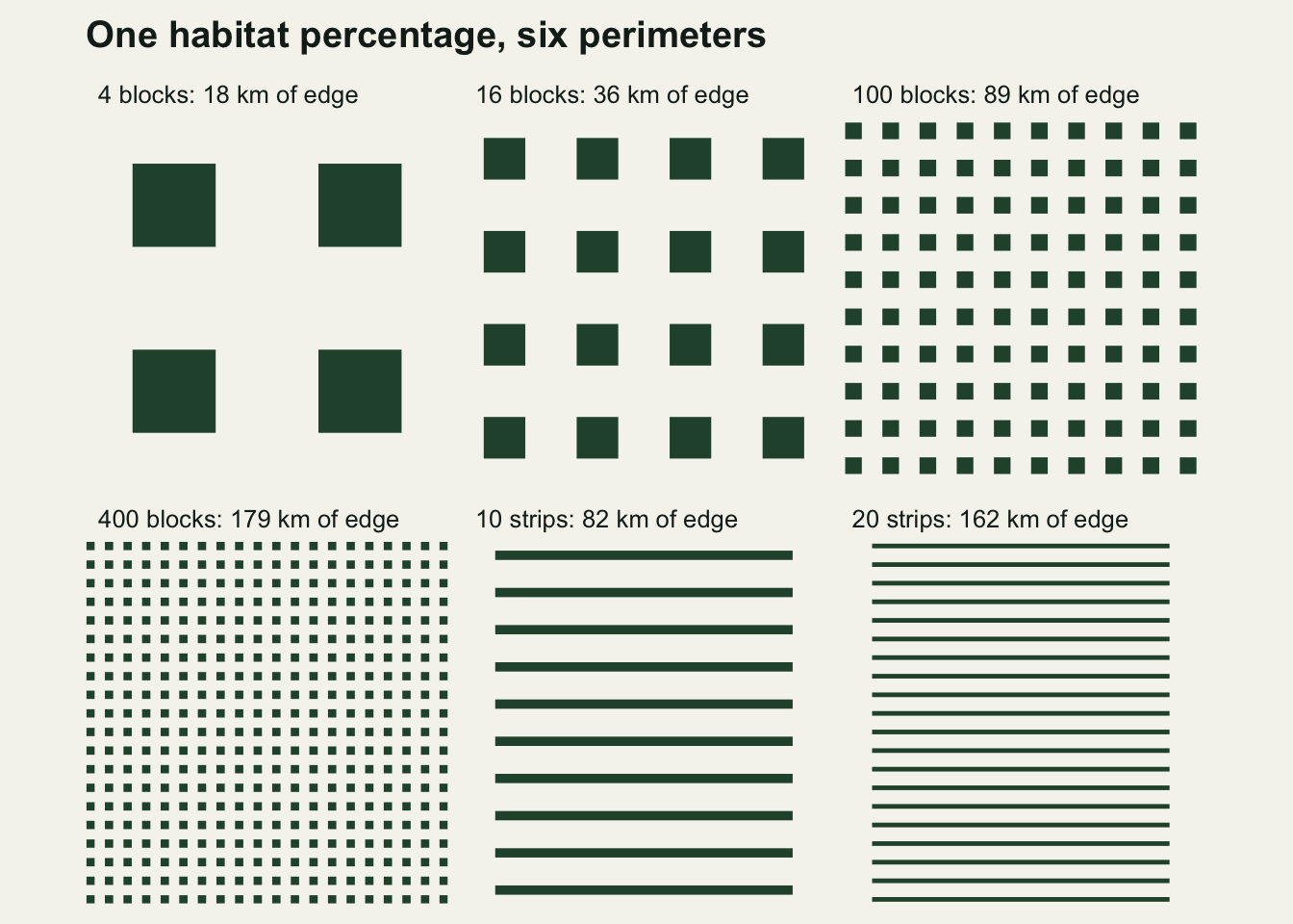
The prediction comes before the simulation. Take a boundary that is locally straight and records spread at a constant density, and displace each record by an isotropic Gaussian of standard deviation sigma. The component of that displacement normal to the boundary is normal with the same standard deviation, so a record sitting a distance d on one side crosses with probability 1 - pnorm(d / sigma). Integrating over all distances gives an expected band of width sigma * dnorm(0) on each side, and both sides contribute, so the expected crossings per unit length of boundary are the record density times sigma * sqrt(2 / pi). Divide by the records in the extent and the expected misassigned share is k * L * sigma / A, with L the boundary length, A the extent area and k a pure number set by the normal distribution. The sweep is what tests it.
n_law <- 40000
sig_grid <- c(5, 10, 25, 50, 100, 250, 500)
lin_cut <- 0.05
small_pred <- k_geom * min(peri) * min(sig_grid) / a_ext
small_rel_se <- sqrt(small_pred * (1 - small_pred) / n_law) / small_pred
arg_all <- as.vector(outer(peri, sig_grid) / a_ext)
arg_lin <- arg_all[k_geom * arg_all < lin_cut]
p_lin <- k_geom * arg_lin
k_se_one <- sqrt(sum(n_law * p_lin * (1 - p_lin))) / sum(n_law * arg_lin)
near_round <- 0.8
round_gap <- abs(k_geom - near_round) / k_se_one
n_sweep <- 12
n_use <- 3000; n_rep <- 30
pref_w <- 4
rep_se <- sqrt(4 / n_use)
mean_se <- rep_se / sqrt(n_rep)
sig_e <- 50; sig_b <- 50
n_acc <- 6; n_place <- 60
share_se <- sqrt(0.25 / n_place)
acc_rad <- 900; unc_fine <- 15; unc_coarse <- 500; unc_cut <- 100
k_side <- 11; n_node <- k_side^2
n_mod <- 20000; n_fix <- 20000; n_soft <- 4000
rate_se <- sqrt(0.25 / (n_mod * hab_frac * pref_w /
                          (hab_frac * pref_w + 1 - hab_frac)))
print(round(c(predicted_constant = k_geom, records_per_cell = n_law,
              smallest_predicted_share = small_pred,
              relative_mc_error_there = small_rel_se,
              pooled_se_of_one_sweep = k_se_one, sweeps = n_sweep,
              se_of_the_sweep_mean = k_se_one / sqrt(n_sweep),
              replicates = n_rep, records_per_replicate = n_use,
              se_of_one_replicate = rep_se, mc_error_of_the_mean = mean_se,
              placements = n_place, worst_se_of_a_share = share_se,
              records_per_error_model = n_mod, worst_se_of_a_rate = rate_se,
              records_for_the_repairs = n_fix, records_for_the_soft_fit = n_soft,
              quadrature_nodes = n_node), 4))
predicted_constant records_per_cell smallest_predicted_share
7.979e-01 4.000e+04 2.900e-03
relative_mc_error_there pooled_se_of_one_sweep sweeps
9.340e-02 8.200e-03 1.200e+01
se_of_the_sweep_mean replicates records_per_replicate
2.400e-03 3.000e+01 3.000e+03
se_of_one_replicate mc_error_of_the_mean placements
3.650e-02 6.700e-03 6.000e+01
worst_se_of_a_share records_per_error_model worst_se_of_a_rate
6.450e-02 2.000e+04 5.000e-03
records_for_the_repairs records_for_the_soft_fit quadrature_nodes
2.000e+04 4.000e+03 1.210e+02 The constant the geometry predicts is 0.7979, and every replication number used below is set in that chunk, which runs before anything stochastic does. The sweep uses 40000 records per cell because the smallest cell has a predicted share of 0.0029, on which that many Bernoulli draws put a Monte Carlo error of 9.3 per cent, while pooling those cells puts the error on the constant at 1.0 per cent of it. That is enough to tell 0.7979 apart from one or from a half, and not enough to tell it apart from 0.8, which sits 0.26 of a standard error away. So the sweep is run 12 times on fresh records, which puts the error of the mean near 0.0024, small enough for a departure of one per cent of the constant to show. The attenuation study uses 30 replicates of 3000 records, because one replicate carries a standard error near 0.037 on a log ratio and that many bring the error of the mean to 0.0067, well below the smallest difference between landscapes that section claims. The misclassification-rate comparison uses 20000 records, leaving at worst 0.5 percentage points of Monte Carlo error on a crossing rate. The filter and buffer repairs use 20000; the filter is replicated over 60 placements of its access points, since placement is the random input there, on which any share is resolved to at worst 6.5 percentage points. The soft-label fit uses 4000, smaller because its comparison evaluates the map at 121 quadrature nodes per record.
set.seed(226201)
base_xy <- cbind(runif(n_law, x_org, x_org + ext_m),
                 runif(n_law, y_org, y_org + ext_m))
true_cl <- lapply(hab, function(h) in_poly(base_xy, h))

set.seed(226202)
law <- do.call(rbind, lapply(seq_along(lay), function(i)
  do.call(rbind, lapply(sig_grid, function(s) {
    obs <- in_poly(shift_by(base_xy, s), hab[[i]])
    data.frame(layer = names(lay)[i], perim = peri[i], sigma = s,
               wrong = sum(obs != true_cl[[i]]))
  }))))
law$layer <- factor(law$layer, levels = names(lay))
law$share <- law$wrong / n_law
law$mc_se <- sqrt(law$share * (1 - law$share) / n_law)
law$arg <- law$perim * law$sigma / a_ext
law$predicted <- k_geom * law$arg
sel <- law$predicted < lin_cut
k_fit <- sum(law$wrong[sel]) / sum(n_law * law$arg[sel])
k_se <- sqrt(sum(n_law * law$share[sel] * (1 - law$share[sel]))) /
  sum(n_law * law$arg[sel])
ceiling_pred <- 2 * hab_frac * (1 - hab_frac)
print(law[sel, c("layer", "sigma", "arg", "share", "mc_se", "predicted")],
      row.names = FALSE, digits = 4)
layer sigma arg share mc_se predicted
4 blocks 5 0.003578 0.002775 0.0002630 0.002855
4 blocks 10 0.007155 0.005500 0.0003698 0.005709
4 blocks 25 0.017889 0.014125 0.0005900 0.014273
4 blocks 50 0.035777 0.028300 0.0008291 0.028546
16 blocks 5 0.007155 0.005650 0.0003748 0.005709
16 blocks 10 0.014311 0.011600 0.0005354 0.011418
16 blocks 25 0.035777 0.028700 0.0008348 0.028546
100 blocks 5 0.017889 0.014700 0.0006017 0.014273
100 blocks 10 0.035777 0.026225 0.0007990 0.028546
400 blocks 5 0.035777 0.029375 0.0008443 0.028546
10 strips 5 0.016500 0.013650 0.0005802 0.013165
10 strips 10 0.033000 0.026625 0.0008049 0.026330
20 strips 5 0.032500 0.025225 0.0007840 0.025931set.seed(226203)
k_rep <- vapply(seq_len(n_sweep), function(r) {
bxy <- cbind(runif(n_law, x_org, x_org + ext_m),
runif(n_law, y_org, y_org + ext_m))
num <- den <- 0
for (i in seq_along(lay)) {
tc <- NULL
for (s in sig_grid[k_geom * peri[i] * sig_grid / a_ext < lin_cut]) {
if (is.null(tc)) tc <- in_poly(bxy, hab[[i]])
num <- num + sum(in_poly(shift_by(bxy, s), hab[[i]]) != tc)
den <- den + n_law * peri[i] * s / a_ext
}
}
num / den
}, 0)
k_bar <- mean(k_rep); k_bar_se <- sd(k_rep) / sqrt(n_sweep)
k_shift_pct <- 100 * (k_geom / k_bar - 1)
print(round(c(cells_used = sum(sel), k_one_sweep = k_fit, k_mc_se = k_se,
k_over_sweeps = k_bar, sd_across_sweeps = sd(k_rep),
mc_error_of_that_mean = k_bar_se, k_predicted = k_geom,
shortfall_pct = 100 * (1 - k_bar / k_geom),
gap_in_mc_errors = abs(k_bar - k_geom) / k_bar_se,
saturation_ceiling = ceiling_pred,
largest_share_seen = max(law$share)), 4)) cells_used k_one_sweep k_mc_se
13.0000 0.7931 0.0081
k_over_sweeps sd_across_sweeps mc_error_of_that_mean
0.7888 0.0126 0.0036
k_predicted shortfall_pct gap_in_mc_errors
0.7979 1.1394 2.4976
saturation_ceiling largest_share_seen
0.3200 0.3120 One sweep fits 0.7931 with a Monte Carlo error of 0.0081; the 12 sweeps average 0.7888 with an error of the mean of 0.0036, against a predicted 0.7979. That is a shortfall of 1.1 per cent, 2.5 standard errors below the prediction, so it is a small systematic effect rather than noise. Its direction is the one the derivation’s approximations force: the law counts crossings per unit of boundary as though the boundary were straight and each record could cross once, while at a convex corner the bands from the two edges overlap and across a narrow patch a record can pass right over and land back in its own class. Both subtract. The law is right to leading order and overpredicts by that much on these geometries. The spread across sweeps, 0.0126, is wider than the 0.0082 a sweep would carry if its cells were independent, because every cell in a sweep is scored on the same records. The 13 cells pooled are the ones whose predicted share was under 0.05, a cut taken from the prediction before any share was computed.
pal_lay <- setNames(c(te_forest, "#4f8f63", te_gold, te_rust, "#7b6ca8", "#3f6f8f"),
                    names(lay))
base_p <- function(xv, ttl, xlab) {
  ggplot(law, aes(.data[[xv]], share, colour = layer)) +
    geom_point(size = 1.9) +
    scale_colour_manual(values = pal_lay, name = NULL) +
    scale_x_log10() + scale_y_log10() +
    labs(x = xlab, y = "share in the wrong class", title = ttl) +
    guides(colour = guide_legend(nrow = 1, override.aes = list(size = 2.6))) +
    theme_datasheet()
}
p_raw <- base_p("sigma", "By coordinate error alone",
                "coordinate error, sigma (metres)")
p_col <- base_p("arg", "Rescaled by perimeter and error", "L * sigma / A") +
  geom_abline(slope = 1, intercept = log10(k_geom), linetype = "dashed",
              colour = te_body, linewidth = 0.6) +
  geom_hline(yintercept = ceiling_pred, linetype = "dotted",
             colour = te_body, linewidth = 0.6)

p_raw + p_col + plot_layout(guides = "collect") +
  plot_annotation(theme = theme_datasheet() +
                    theme(legend.position = "bottom"))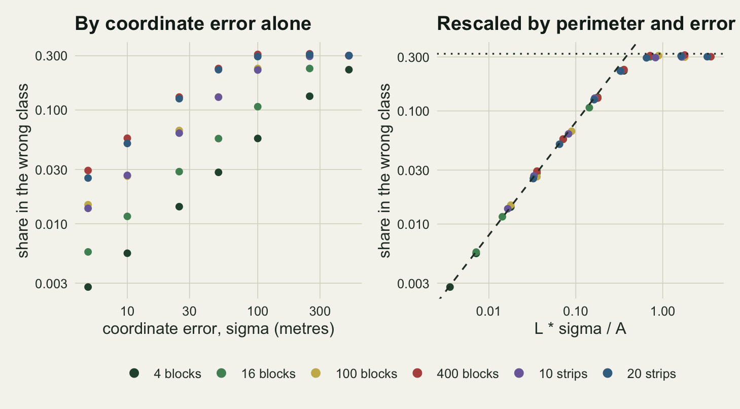
Two features of the right-hand panel are worth naming. The strips and the block lattices lie on the same line, so the constant does not care whether the habitat is compact or elongated, only how much edge it carries. And the line ends: past an argument of about one the points bend onto a ceiling at 0.32, the largest share observed being 0.312. That ceiling is not an artefact. Once the error is large compared with the patches the recorded position carries no information about the true class, and two independent draws from a landscape that is 20 per cent habitat disagree that often. Naimi and colleagues (2014) reached the qualitative version by simulating across landscapes: positional uncertainty bites where the environment turns over quickly in space. The arithmetic above says how quickly, in units anyone can read off a shapefile.
The same target precision costs ten times more in a fragmented landscape
The law is more useful upside down. Fix the misassignment rate you are willing to tolerate and solve for the coordinate error that delivers it: sigma = q_tol * A / (k * L). The tolerance is a decision and the other two are read off the map before a record has been downloaded; only the constant comes from somewhere else, and the table below uses the measured 0.7888 rather than the derived 0.7979, which moves every entry by 1.2 per cent.
targets <- c(0.01, 0.05, 0.10)
need <- data.frame(layer = names(lay), perimeter_km = peri / 1000)
for (q_tol in targets)
  need[[sprintf("sigma_for_%.0f_pct", 100 * q_tol)]] <-
    round(q_tol * a_ext / (k_bar * peri), 1)
print(need, row.names = FALSE)
layer perimeter_km sigma_for_1_pct sigma_for_5_pct sigma_for_10_pct
4 blocks 17.88854 17.7 88.6 177.2
16 blocks 35.77709 8.9 44.3 88.6
100 blocks 89.44272 3.5 17.7 35.4
400 blocks 178.88544 1.8 8.9 17.7
10 strips 82.50000 3.8 19.2 38.4
20 strips 162.50000 2.0 9.8 19.5need_5 <- setNames(targets[2] * a_ext / (k_bar * peri), names(lay))
by_sim <- vapply(c("4 blocks", "400 blocks"), function(nm) {
d <- law[law$layer == nm, ]
approx(d$share, d$sigma, xout = targets[2])$y
}, 0)
print(round(c(law_compact = need_5[["4 blocks"]],
simulation_compact = by_sim[["4 blocks"]],
law_fragmented = need_5[["400 blocks"]],
simulation_fragmented = by_sim[["400 blocks"]],
ratio = need_5[["4 blocks"]] / need_5[["400 blocks"]]), 2)) law_compact simulation_compact law_fragmented
88.59 88.89 8.86
simulation_fragmented ratio
8.81 10.00 For a tolerance of 5 per cent misassigned, the four-block landscape needs coordinates good to 89 metres and the four-hundred-block landscape needs 8.9 metres, a ratio of 10. The first is an ordinary phone fix in the open. The second is a differential correction or a location that was mapped rather than measured, and it is out of reach for most aggregator records. Reading the required precision straight off the simulated curves instead of off the law gives 89 and 8.8 metres, the same answer arrived at the expensive way. The two tightest rows in the table are that four-hundred-block layer and the twenty-strip layer at 9.8 metres, and they are tight for the same reason: they carry the most boundary. What the strips add is that a landscape does not have to look shattered to get there. Twenty parallel strips are a landscape most readers would call simple, they hold exactly as much habitat as the four blocks, and they demand coordinates 9 times better. Linear habitat is what a great deal of conservation work is about, from hedgerows and riparian strips to verges and ditches.
The damage is attenuation, and almost all of it comes from the edges
A misassignment rate is only interesting through what it does to an estimate. The estimate here is the plainest habitat preference there is: a log selection ratio, the odds that a record sits in habitat divided by the odds that a random point does. Records are generated at a density 4 times higher in habitat than in the matrix, so the true value is the log of that. Every level of error is applied to the same record pool, so the curves are paired and their shape is not confounded with resampling noise.
draw_used <- function(h, n_want, seed, gfun = NULL, b = NULL) {
  set.seed(seed); out <- matrix(0, 0, 2)
  while (nrow(out) < n_want) {
    m <- cbind(runif(2 * n_want, x_org, x_org + ext_m),
               runif(2 * n_want, y_org, y_org + ext_m))
    m <- m[in_poly(m, h) | runif(nrow(m)) < 1 / pref_w, , drop = FALSE]
    if (!is.null(gfun)) m <- m[runif(nrow(m)) < gfun(edge_gap(m, b)), , drop = FALSE]
    out <- rbind(out, m)
  }
  out[seq_len(n_want), , drop = FALSE]
}
beta_of <- function(o, la = lg_avail) log(sum(o) / sum(!o)) - la
sig_att <- c(0, 5, 10, 25, 50, 100, 250)
att <- do.call(rbind, lapply(c("4 blocks", "400 blocks"), function(nm) {
  pool <- draw_used(hab[[nm]], n_use * n_rep, 226300 + which(nm == names(lay)))
  set.seed(226310)
  do.call(rbind, lapply(sig_att, function(s) {
    obs <- in_poly(if (s == 0) pool else shift_by(pool, s), hab[[nm]])
    bs <- vapply(seq_len(n_rep), function(r)
      beta_of(obs[((r - 1) * n_use + 1):(r * n_use)]), 0)
    data.frame(layer = nm, sigma = s, beta = mean(bs), mc_se = sd(bs) / sqrt(n_rep))
  }))
}))
att$intact <- ave(att$beta, att$layer, FUN = function(v) v[1])
att$kept <- att$beta / att$intact
att$kept_se <- att$mc_se / abs(att$intact)
print(att[, c("layer", "sigma", "beta", "mc_se", "kept")],
      row.names = FALSE, digits = 4)
layer sigma beta mc_se kept
4 blocks 0 1.38825 0.005771 1.00000
4 blocks 5 1.37731 0.005779 0.99212
4 blocks 10 1.36789 0.005777 0.98533
4 blocks 25 1.33280 0.005512 0.96006
4 blocks 50 1.28177 0.005960 0.92330
4 blocks 100 1.17646 0.005422 0.84744
4 blocks 250 0.88711 0.005402 0.63901
400 blocks 0 1.39395 0.007820 1.00000
400 blocks 5 1.28461 0.007741 0.92156
400 blocks 10 1.18164 0.007306 0.84769
400 blocks 25 0.89379 0.006980 0.64120
400 blocks 50 0.45676 0.007935 0.32768
400 blocks 100 0.02272 0.007768 0.01630
400 blocks 250 -0.10258 0.008448 -0.07359cmp <- att[att$sigma == sig_e, ]
flat <- att[att$layer == "400 blocks" & att$sigma == 100, ]At an error of 50 metres, which is an ordinary handheld fix, the compact landscape keeps 92.3 per cent of the coefficient and the fragmented one keeps 32.8 per cent. At 100 metres the fragmented estimate is 0.023 with a Monte Carlo error of 0.008, which is 1.6 per cent of what the same records return with exact coordinates, on a landscape where the butterfly really is 4 times as dense in the meadows. Graham and colleagues (2008) found the same direction of travel in distribution models built on displaced occurrence records, and this is the mechanism underneath it: the label, not the covariate, is what the error destroys.
ggplot(att[att$sigma > 0, ], aes(sigma, kept, colour = layer)) +
  geom_hline(yintercept = 1, colour = te_body, linewidth = 0.4) +
  geom_hline(yintercept = 0, linetype = "dashed", colour = te_body,
             linewidth = 0.4) +
  geom_line(linewidth = 0.8) +
  geom_errorbar(aes(ymin = kept - kept_se, ymax = kept + kept_se), width = 0.04,
                linewidth = 0.5) +
  geom_point(size = 2.6) +
  scale_colour_manual(values = c("4 blocks" = te_forest,
                                 "400 blocks" = te_rust), name = NULL) +
  scale_x_log10() +
  labs(x = "coordinate error, sigma (metres)",
       y = "share of the preference retained",
       title = "The same coordinates, two landscapes",
       subtitle = "identical habitat percentage, ten times the edge") +
  theme_datasheet() + theme(legend.position = "bottom")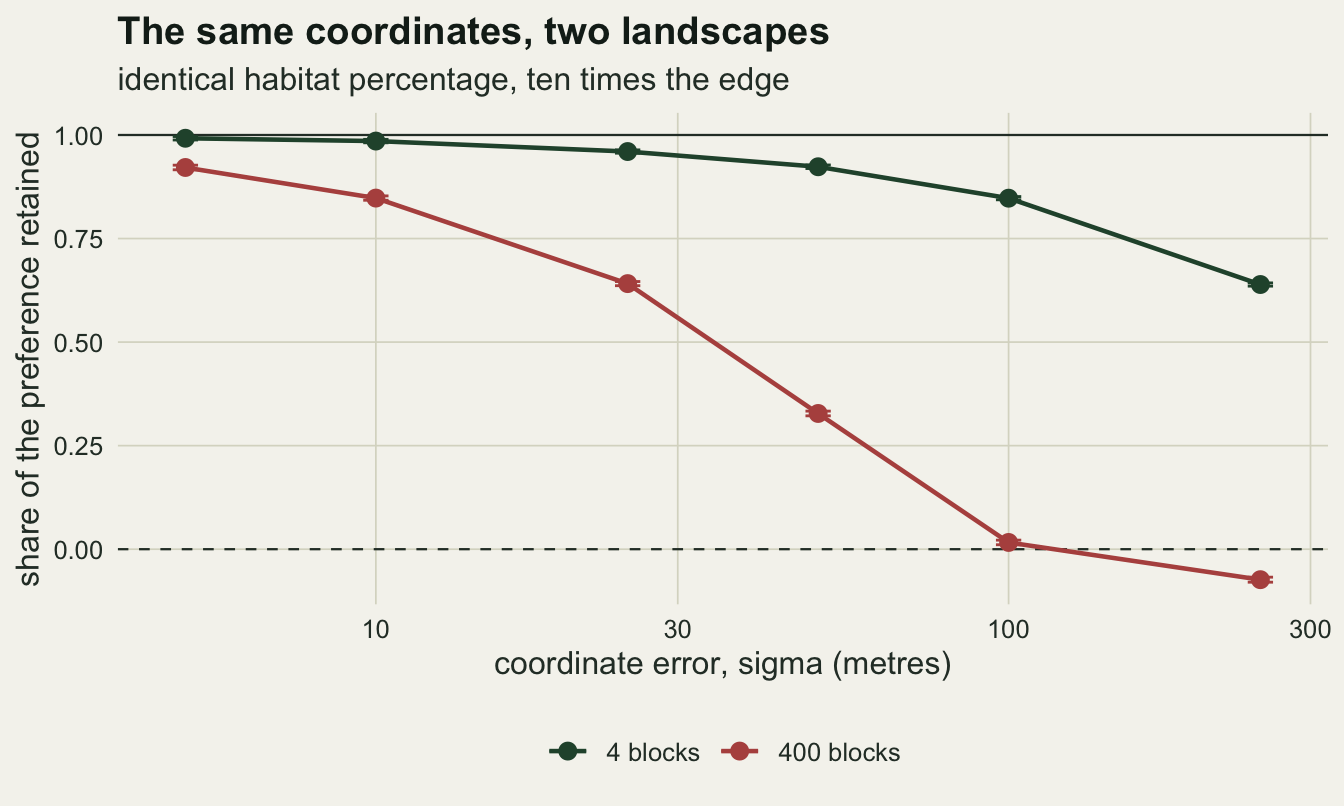
What separates this from ordinary misclassification is where the errors sit. A record in the middle of a meadow is not at risk at any plausible coordinate error; a record near an edge is at risk of nothing else. Taking the compact layer at 50 metres of error and splitting the records by their true distance to the nearest boundary makes the profile visible.
nm_e <- "4 blocks"
set.seed(226320)
true_e <- true_cl[[nm_e]]
gap_e <- edge_gap(base_xy, bnd[[nm_e]])
wrong_e <- in_poly(shift_by(base_xy, sig_e), hab[[nm_e]]) != true_e
near <- gap_e <= sig_e
brk <- c(0, 12.5, 25, 50, 75, 100, 150, 250, Inf)
gp <- cut(gap_e, brk, right = FALSE)
prof <- data.frame(mid = vapply(split(gap_e, gp), mean, 0),
                   n = as.numeric(table(gp)),
                   share = vapply(split(wrong_e, gp), mean, 0))
prof$mc_se <- sqrt(prof$share * (1 - prof$share) / prof$n)
prof$at_mid <- 1 - pnorm(prof$mid / sig_e)
prof$theory <- vapply(split(gap_e, gp), function(v) mean(1 - pnorm(v / sig_e)), 0)
prof$z <- ifelse(prof$mc_se > 0, (prof$share - prof$theory) / prof$mc_se, NA)
print(prof, digits = 4)
mid n share mc_se at_mid theory z
[0,12.5) 6.364 713 0.4291725 0.0185363 4.494e-01 4.495e-01 -1.09551
[12.5,25) 18.401 683 0.3587116 0.0183522 3.564e-01 3.568e-01 0.10505
[25,50) 37.741 1464 0.2370219 0.0111142 2.252e-01 2.275e-01 0.85406
[50,75) 62.604 1481 0.1033086 0.0079088 1.053e-01 1.077e-01 -0.54947
[75,100) 87.510 1387 0.0504686 0.0058780 4.004e-02 4.165e-02 1.50048
[100,150) 124.905 2829 0.0084836 0.0017243 6.243e-03 8.153e-03 0.19178
[150,250) 199.969 5570 0.0001795 0.0001795 3.176e-05 1.900e-04 -0.05852
[250,Inf) 501.407 25873 0.0000000 0.0000000 0.000e+00 5.675e-09 NAres_z <- prof$z[!is.na(prof$z)]
lift_pct <- 100 * (prof$theory / prof$at_mid - 1); far <- 6L
outer_half <- gap_e > median(gap_e)
print(round(c(records_within_one_sigma = mean(near),
band_share_predicted = unname(2 * peri[nm_e] * sig_e / a_ext),
errors_from_within_one_sigma = mean(near[wrong_e]),
overall_share_wrong = mean(wrong_e),
records_in_the_outer_half = sum(outer_half),
wrong_in_the_outer_half = sum(wrong_e & outer_half)), 4)) records_within_one_sigma band_share_predicted
7.150e-02 7.160e-02
errors_from_within_one_sigma overall_share_wrong
7.836e-01 2.860e-02
records_in_the_outer_half wrong_in_the_outer_half
2.000e+04 0.000e+00 The band within one standard deviation of a boundary holds 7.1 per cent of the records, close to the 7.2 per cent the geometry predicts, and it supplies 78.4 per cent of all the misassignments. In the outer half of the block, meaning every record more than 358 metres from any boundary, 0 records out of 20000 were misassigned. The profile is the function the derivation started from, 1 - pnorm(d / sigma), but comparing a binned share with it takes one step of care: that function is convex, so its average over a bin sits above its value at the bin’s mean distance, by 31 per cent in the bin from 100 to 150 metres. Evaluated at that one distance it would run below the far bins for that reason alone. Averaged over the records in each bin instead, it sits within 1.5 Monte Carlo errors of every observed share, with the share above the curve in 4 of the 7 bins in which any record was misassigned at all.
cum_d <- data.frame(d = sort(gap_e[wrong_e]) / sig_e)
cum_d$share <- seq_len(nrow(cum_d)) / nrow(cum_d)
p_prof <- ggplot(prof, aes(mid, share)) +
  geom_line(aes(y = theory), linetype = "dashed", colour = te_body,
            linewidth = 0.6) +
  geom_errorbar(aes(ymin = share - mc_se, ymax = share + mc_se), width = 4,
                colour = te_forest, linewidth = 0.5) +
  geom_point(size = 2.4, colour = te_forest) +
  coord_cartesian(xlim = c(0, 250)) +
  labs(x = "true distance to a boundary (metres)",
       y = "probability of the wrong class", title = "Risk lives in a band") +
  theme_datasheet()
p_cum <- ggplot(cum_d, aes(d, share)) +
  geom_vline(xintercept = 1, linetype = "dotted", colour = te_body,
             linewidth = 0.5) +
  geom_line(colour = te_rust, linewidth = 0.9) +
  coord_cartesian(xlim = c(0, 3.1)) +
  labs(x = "distance to a boundary, in units of sigma",
       y = "cumulative share of the misassignments",
       title = "And it is a thin band") +
  theme_datasheet()

p_prof + p_cum + plot_annotation(theme = theme_datasheet())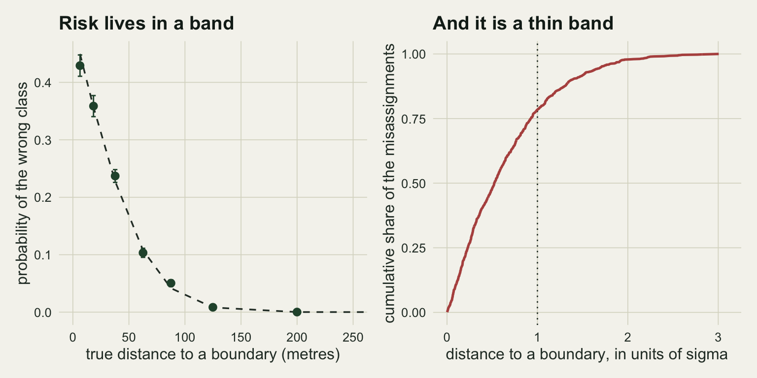
That concentration is what stops the textbook repair working unchanged. Non-differential misclassification of a binary exposure attenuates an odds ratio by a factor set by the two error rates, and Copeland and colleagues (1977) give the inversion: with the rates in hand the observed counts can be pushed back to the true ones. Those rates look computable from the map here, since the share of habitat records that cross out is k * sigma * L / (2 * A_h) and the share of matrix records that cross in is the same expression with the matrix area underneath. What the correction needs, though, is the rate for the records in the dataset, a property of where the animals were rather than of the map. Three record sets on one layer settle it: one spread evenly within each class, one avoiding edges, one seeking them.
nm_m <- "100 blocks"; d_scale <- 40
mods <- list(even = NULL, "avoids edges" = function(d) 1 - exp(-d / d_scale),
             "seeks edges" = function(d) exp(-d / d_scale))
sig_m <- c(0, 25)
back_out <- function(p_obs, a, b) {
  th <- (p_obs - b) / (1 - a - b)
  log(th / (1 - th)) - lg_avail
}
mres <- do.call(rbind, lapply(names(mods), function(mn) {
  pool <- draw_used(hab[[nm_m]], n_mod, 226330 + which(mn == names(mods)),
                    mods[[mn]], bnd[[nm_m]])
  tcl <- in_poly(pool, hab[[nm_m]])
  set.seed(226340)
  do.call(rbind, lapply(sig_m, function(s) {
    obs <- if (s == 0) tcl else in_poly(shift_by(pool, s), hab[[nm_m]])
    data.frame(model = mn, sigma = s, n_hab = sum(tcl),
               out_rate = mean(!obs[tcl]), in_rate = mean(obs[!tcl]),
               out_se = sqrt(mean(!obs[tcl]) * mean(obs[tcl]) / sum(tcl)),
               out_map = k_geom / 2 * s * peri[nm_m] / a_hab,
               in_map = k_geom / 2 * s * peri[nm_m] / a_mat,
               beta = beta_of(obs), beta_se = sqrt(1 / sum(obs) + 1 / sum(!obs)))
  }))
}))
mres$beta_intact <- ave(mres$beta, mres$model, FUN = function(v) v[1])
mres$corrected <- ifelse(mres$sigma == 0, mres$beta,
                         back_out(plogis(mres$beta + lg_avail), mres$out_map,
                                  mres$in_map))
mres$lost_pct <- 100 * (1 - mres$beta / mres$beta_intact)
mres$miss_pct <- 100 * (mres$corrected / mres$beta_intact - 1)
print(mres[, c("model", "sigma", "n_hab", "out_rate", "out_se", "out_map",
               "beta", "beta_se", "corrected", "lost_pct", "miss_pct")],
      row.names = FALSE, digits = 4)
model sigma n_hab out_rate out_se out_map beta beta_se corrected
even 0 9994 0.00000 0.000000 0.0000 1.3851 0.01414 1.3851
even 25 9994 0.17120 0.003768 0.1784 1.1273 0.01426 1.3992
avoids edges 0 8060 0.00000 0.000000 0.0000 0.9933 0.01442 0.9933
avoids edges 25 8060 0.08474 0.003102 0.1784 0.8889 0.01458 1.1015
seeks edges 0 13694 0.00000 0.000000 0.0000 2.1618 0.01522 2.1618
seeks edges 25 13694 0.26369 0.003765 0.1784 1.5813 0.01421 1.9994
lost_pct miss_pct
0.00 0.000
18.62 1.018
0.00 0.000
10.51 10.894
0.00 0.000
26.85 -7.508hit <- mres[mres$sigma == max(sig_m), ]
even_gap_pct <- 100 * (hit$out_map[1] / hit$out_rate[1] - 1)
even_gap_z <- (hit$out_map[1] - hit$out_rate[1]) / hit$out_se[1]At 25 metres of error on this layer the map predicts that 17.8 per cent of habitat records cross out. The evenly spread set delivers 17.1 per cent, with a Monte Carlo error of 0.4 percentage points on it: for records with no relation to the edges the map-derived rate is 4.2 per cent of itself too high, a gap of 1.9 Monte Carlo errors. So the map is right to a few per cent there, and this run cannot say whether the small residual is the shortfall the sweep found in the constant or noise. The edge-avoiding set delivers 8.5 per cent, so the map overstates its rate by a factor of 2.11, and the edge-seeking set delivers 26.4 per cent, so the map understates by a factor of 1.48.
Pushing those through the correction shows what the difference costs. Uncorrected, the three sets lose 18.6, 10.5 and 26.9 per cent of their own error-free coefficient. Corrected with the map-derived rates they miss that coefficient by +1.0, +10.9 and -7.5 per cent. So the correction does transfer, and it transfers well for records that ignore the edges; on the other two it leaves a residual of the order of a tenth of the coefficient, and the residual changes sign. The map buys an approximate rate, and an approximate rate buys an approximate correction.
Three repairs, and the price of each
The first repair is the one the aggregator invites: filter on the reported coordinate uncertainty and keep the good records. The cost is not only sample size. Precise records are made by people standing in places people go, and where people go is not a random sample of the landscape. The set-up below puts 6 access points in the matrix, gives records within 900 metres of one of them an uncertainty of 15 metres and everything else 500 metres, then filters at 100 metres. Where the access points fall is the dominant random input, not the records, so one placement is one draw from the experiment and the whole thing is run 60 times on one fixed pool of records.
nm_f <- "4 blocks"
pool_f <- draw_used(hab[[nm_f]], n_fix, 226450)
true_f <- in_poly(pool_f, hab[[nm_f]])
truth_f <- beta_of(true_f)
set.seed(226440)
one_place <- function(r) {
  acc_xy <- matrix(0, 0, 2)
  while (nrow(acc_xy) < n_acc) {
    m <- cbind(runif(30, x_org, x_org + ext_m), runif(30, y_org, y_org + ext_m))
    acc_xy <- rbind(acc_xy, m[!in_poly(m, hab[[nm_f]]), , drop = FALSE])
  }
  acc_xy <- acc_xy[seq_len(n_acc), ]
  gap_acc <- sqrt(apply(outer(pool_f[, 1], acc_xy[, 1], "-")^2 +
                          outer(pool_f[, 2], acc_xy[, 2], "-")^2, 1, min))
  reported <- ifelse(gap_acc <= acc_rad, unc_fine, unc_coarse)
  obs_f <- in_poly(cbind(pool_f[, 1] + rnorm(n_fix, 0, reported),
                         pool_f[, 2] + rnorm(n_fix, 0, reported)), hab[[nm_f]])
  kept_f <- reported <= unc_cut
  data.frame(place = r, records_kept = mean(kept_f),
             all_records = beta_of(obs_f), filtered = beta_of(obs_f[kept_f]),
             selection_only = beta_of(true_f[kept_f]),
             within_se = sqrt(1 / sum(true_f[kept_f]) +
                                1 / sum(!true_f[kept_f])))
}
plc <- do.call(rbind, lapply(seq_len(n_place), one_place))
filt <- do.call(rbind, lapply(c("all_records", "filtered", "selection_only"),
  function(cn) data.frame(quantity = cn, mean = mean(plc[[cn]]),
                          sd_across_placements = sd(plc[[cn]]),
                          se_of_mean = sd(plc[[cn]]) / sqrt(n_place),
                          pct_below_truth = 100 * mean(plc[[cn]] < truth_f))))
print(filt, row.names = FALSE, digits = 4)
quantity mean sd_across_placements se_of_mean pct_below_truth
all_records 0.7695 0.1083 0.01398 100.00
filtered 1.1635 0.2673 0.03451 78.33
selection_only 1.1982 0.2664 0.03439 76.67print(round(c(truth = truth_f,
truth_se = sqrt(1 / sum(true_f) + 1 / sum(!true_f)),
mean_records_kept = mean(plc$records_kept),
mean_within_placement_se = mean(plc$within_se),
placements = n_place), 4)) truth truth_se mean_records_kept
1.3943 0.0141 0.3865
mean_within_placement_se placements
0.0232 60.0000 Keeping only the precise records throws away 61 per cent of the data and moves the estimate from 0.770 to 1.164 on average, against a truth of 1.394: most of the attenuation goes, and most of what is left is not measurement error. Given exact coordinates the retained records alone return 1.198 averaged over placements, 14.1 per cent below the truth, and they fall below it in 77 per cent of the placements. The filter trades a large downward bias for a smaller one of the same sign, because the retained records report on a neighbourhood of the access points rather than on the block.
That direction is a tendency and not a rule, which is why the placement is replicated. Across placements the selection-only estimate has a standard deviation of 0.266, about 11 times the 0.023 standard error any one of them carries within itself: run once, this experiment reports a precision that describes the wrong source of variation, and it can land either side of the truth. Averaging pins the mean down to 0.034. The filter is still worth running, and it has to be followed by redefining availability over the area the surviving records actually sample, the point Barry and Elith (2006) make about the difference between the data an ecologist has and the population a habitat model is written about.
The second repair works on the geometry: buffer the class boundaries and drop every record whose recorded position falls inside the buffer. Availability has to be recomputed on the eroded map, or the repair introduces a worse bias than the one it removes. Recomputing it also settles what the repair is aiming at, which is the selection ratio of the eroded map: the value an analyst with exact coordinates would get from the records whose true positions survive the same buffer. That value does not drift as the buffer widens, because eroding a map does not change how much denser the records are inside habitat than out.
buf_tab <- do.call(rbind, lapply(c("100 blocks", "400 blocks"), function(nm) {
  pool <- draw_used(hab[[nm]], n_fix, 226400 + which(nm == names(lay)))
  tcl <- in_poly(pool, hab[[nm]]); gap_t <- edge_gap(pool, bnd[[nm]])
  set.seed(226410)
  moved <- shift_by(pool, sig_b)
  ocl <- in_poly(moved, hab[[nm]]); gap_o <- edge_gap(moved, bnd[[nm]])
  do.call(rbind, lapply(c(0, 1, 2), function(mult) {
    wd <- mult * sig_b; keep <- gap_o > wd; core <- gap_t > wd
    ah <- if (wd == 0) a_hab else
      sum(as.numeric(st_area(st_buffer(hab[[nm]], -wd))))
    am <- if (wd == 0) a_mat else
      sum(as.numeric(st_area(st_difference(blk, st_buffer(hab[[nm]], wd)))))
    ok <- sum(keep) > 50 && ah > 0 && am > 0
    okc <- ok && sum(tcl[core]) > 0 && sum(!tcl[core]) > 0
    data.frame(layer = nm, buffer_m = wd, kept = mean(keep),
               habitat_core_pct = 100 * ah / a_hab,
               estimate = if (ok) beta_of(ocl[keep], log(ah / am)) else NA,
               beta_se = if (ok) sqrt(1 / sum(ocl[keep]) +
                                        1 / sum(!ocl[keep])) else NA,
               target = if (okc) beta_of(tcl[core], log(ah / am)) else NA,
               target_se = if (okc) sqrt(1 / sum(tcl[core]) +
                                           1 / sum(!tcl[core])) else NA)
  }))
}))
buf_tab$naive <- ave(buf_tab$estimate, buf_tab$layer, FUN = function(v) v[1])
buf_tab$closed_pct <- 100 * (buf_tab$estimate - buf_tab$naive) /
  (buf_tab$target - buf_tab$naive)
buf_tab$left_se <- (buf_tab$target - buf_tab$estimate) / buf_tab$beta_se
print(buf_tab[, setdiff(names(buf_tab), "naive")], row.names = FALSE, digits = 4)
layer buffer_m kept habitat_core_pct estimate beta_se target target_se
100 blocks 0 1.00000 100.000 0.8808 0.01460 1.389 0.01414
100 blocks 50 0.53910 30.557 1.1907 0.02212 1.395 0.02139
100 blocks 100 0.21125 1.115 1.1947 0.10324 1.323 0.09840
400 blocks 0 1.00000 100.000 0.4473 0.01573 1.393 0.01414
400 blocks 50 0.25815 1.115 0.7524 0.11556 1.386 0.09624
400 blocks 100 0.00445 0.000 NA NA NA NA
closed_pct left_se
0.00 34.837
60.26 9.238
70.94 1.245
0.00 60.104
32.50 5.484
NA NAWith no buffer that target is the ordinary one: the true labels on the whole sample give 1.389, against a generating value of 1.386. On the middling layer a buffer of one standard deviation discards 46 per cent of the records and moves the estimate from 0.881 to 1.191 against a target of 1.395, closing 60 per cent of the gap and stopping 9.2 of its own standard errors short. Widening to two standard deviations leaves 1.1 per cent of the habitat area eligible: the estimate hardly moves, to 1.195, while the standard error grows from 0.015 to 0.103, so the residual that is left, 1.2 standard errors, is no longer separable from noise; the larger closure figure in that row comes from the target, which the thinner core estimates less precisely, and not from the estimate. On the fragmented layer the same one-standard-deviation buffer keeps 26 per cent of the records over 1.1 per cent of the habitat, closes 32 per cent of the gap and returns 0.752, still 5.5 standard errors below its target of 1.386; at two standard deviations there is no core left and no estimate to make. The buffer removes part of the bias on both layers and all of it on neither, and the width that would remove more is the width that erodes the map away.
The third repair keeps every record and stops pretending the class is known. For each recorded position, integrate the error distribution over the map to get the probability mass falling in habitat and the mass falling in the matrix, then fit the preference by maximum likelihood on those masses instead of on a hard label. How that integral is computed matters more than it looks. These layers are axis-aligned rectangles, so the mass of a Gaussian kernel inside a patch is the product of two normal increments and the mass in habitat is the sum of those products over patches: exact, and one line of pnorm. The obvious alternative, a fixed grid of 121 nodes at equally spaced normal quantiles in each axis, is also computed here so that the two can be compared on the same records.
rect_of <- function(g) t(vapply(g, function(p) {
  ring <- p[[1]]
  c(min(ring[, 1]), min(ring[, 2]), max(ring[, 1]), max(ring[, 2]))
}, numeric(4)))
kern_mass <- function(m, rects, s) {
  out <- numeric(nrow(m))
  for (rw in seq_len(nrow(rects)))
    out <- out +
      (pnorm((rects[rw, 3] - m[, 1]) / s) - pnorm((rects[rw, 1] - m[, 1]) / s)) *
      (pnorm((rects[rw, 4] - m[, 2]) / s) - pnorm((rects[rw, 2] - m[, 2]) / s))
  out
}
fit_soft <- function(mh, mm) {
  use <- mh + mm > 0
  nll <- function(bv) -(sum(log(exp(bv) * mh[use] + mm[use])) -
                          sum(use) * log(exp(bv) * a_hab + a_mat))
  bhat <- optimize(nll, c(-3, 6), tol = 1e-8)$minimum
  curv <- (nll(bhat + 1e-3) - 2 * nll(bhat) + nll(bhat - 1e-3)) / 1e-6
  c(bhat, 1 / sqrt(curv), sum(!use))
}
ext_rect <- rect_of(blk)
nodes <- qnorm((seq_len(k_side) - 0.5) / k_side)
off_gr <- expand.grid(dx = nodes, dy = nodes)
in_ext <- function(m) m[, 1] >= x_org & m[, 1] <= x_org + ext_m &
  m[, 2] >= y_org & m[, 2] <= y_org + ext_m
soft_tab <- do.call(rbind, lapply(c("100 blocks", "400 blocks"), function(nm) {
  pool <- draw_used(hab[[nm]], n_soft, 226420 + which(nm == names(lay)))
  tcl <- in_poly(pool, hab[[nm]])
  set.seed(226430)
  moved <- shift_by(pool, sig_b)
  m_hab <- kern_mass(moved, rect_of(lay[[nm]]), sig_b)
  m_mat <- kern_mass(moved, ext_rect, sig_b) - m_hab
  ex <- fit_soft(m_hab, m_mat)
  g_hab <- g_mat <- numeric(n_soft)
  for (nd in seq_len(nrow(off_gr))) {
    z <- cbind(moved[, 1] + sig_b * off_gr$dx[nd],
               moved[, 2] + sig_b * off_gr$dy[nd])
    ih <- in_poly(z, hab[[nm]])
    g_hab <- g_hab + ih; g_mat <- g_mat + (in_ext(z) & !ih)
  }
  qd <- fit_soft(g_hab / nrow(off_gr), g_mat / nrow(off_gr))
  data.frame(layer = nm, truth = beta_of(tcl),
             hard_label = beta_of(in_poly(moved, hab[[nm]])),
             uncertain_class = ex[1], curv_se = ex[2], dropped = ex[3],
             on_node_grid = qd[1], grid_dropped = qd[3])
}))
print(soft_tab, row.names = FALSE, digits = 4)
layer truth hard_label uncertain_class curv_se dropped on_node_grid
100 blocks 1.344 0.8358 1.323 0.04327 0 1.288
400 blocks 1.364 0.4505 1.432 0.07807 0 1.386
grid_dropped
2
2On the middling layer the hard label returns 0.836 against a truth of 1.344, and the uncertain-class fit returns 1.323 with a standard error of 0.043. On the fragmented layer, where the hard label had collapsed to 0.450, it returns 1.432 against a truth of 1.364. It drops 0 records, so it does keep the whole sample, and it pays for the uncertainty in the interval rather than in the point estimate, which is the right place.
The node grid is worth a paragraph of its own, because it is what most people would write. It is deterministic and adds no Monte Carlo error, and it is still wrong: on the same records it returns 1.288 and 1.386, low by 0.035 and 0.046 against the exact masses. Those gaps are 82 and 59 per cent of the standard error each fit reports, and unlike that standard error they do not shrink when the sample grows. The function being integrated is an indicator, discontinuous at every patch edge, and a quadrature rule built for smooth integrands has no error bound on it: trading random error for deterministic error is not the same as removing it. The assumption the whole repair runs on is the one to be most suspicious of, that the error is the size the record says it is.
What to report
Give the total boundary length of the habitat layer alongside the habitat percentage. It is one call to st_length on the boundary, and it is the number that decides whether the coordinates in hand are good enough. A methods section with the percentage and no perimeter has withheld the relevant quantity.
Give the distribution of reported coordinate uncertainty, not a single filter threshold. The threshold is a decision, interpretable only next to the precision the map demands at the tolerance chosen, which the inversion in the second section computes in one line.
Say whether the species has anything to do with edges. An ecotone specialist and an interior species can carry identical reported coordinate uncertainty on identical maps and suffer misassignment rates that differ by a factor of three, and no diagnostic run on the map alone will separate them.
If records were dropped by a filter or by a buffer, recompute availability over the ground the surviving records actually sample, and report the attenuated estimate next to whatever correction was applied, with the error rates that correction used and where they came from. Both repairs change what the sample is about, and a corrected coefficient with no statement of its assumed rates cannot be checked by anyone.
Honest limits
The error model is an isotropic Gaussian with a known standard deviation, the friendliest case there is. Zandbergen (2008) shows that positional error in real spatial data is routinely non-normal and heavy-tailed, with a small fraction of records displaced much further than any fitted standard deviation suggests. A heavy tail moves records across several patches rather than one boundary, which pushes the misassignment rate towards the saturation ceiling faster than the linear law predicts. The geometric constant is specific to the normal distribution; the structural claim, that the rate scales with perimeter times a length scale of the error divided by area, survives any error distribution with a finite mean absolute displacement.
The habitat layers are rectangles on regular lattices, chosen so that perimeter could be varied while area was held exactly fixed. Real patch boundaries are crenulated, so their measured perimeter depends on the digitising scale, and the perimeter driving this law is therefore not a fixed property of the ground either: a more finely digitised map has more perimeter and will demand better coordinates, without the habitat having changed. The rectangles are also what makes the kernel mass in the third repair exact. On a real map that integral has to be done numerically, over an indicator function with a discontinuity at every boundary, and the size of its error has to be measured against a case where the answer is known rather than assumed from the node count.
The reported uncertainty is treated as correct throughout, and in an aggregator download it frequently is not. A blank field is common, a placeholder copied across a whole dataset is common, and a value derived from a gazetteer describes the size of a named place rather than the precision of a fix. The third repair is hurt most, since it takes the reported number as the width of the integration kernel; a systematically understated uncertainty leaves it confident and still biased.
The estimand is a two-class selection ratio with availability known exactly from the map, records are independent given their class, and detection is perfect. Real habitat maps carry their own classification error, which compounds with the coordinate error rather than cancelling it, and real analyses use more than two classes, where a displaced record lands in whichever class happens to be adjacent rather than in a single alternative. Nothing measured here says which way a multi-class version of the bias runs, and nothing here counts the extent boundary itself, which in a study area cut out of a larger landscape is a source of misassignment the perimeter of the habitat layer does not include.
References
Wieczorek J, Guo Q, Hijmans RJ 2004 International Journal of Geographical Information Science 18(8):745-767 (10.1080/13658810412331280211)
Graham CH, Elith J, Hijmans RJ, Guisan A, Peterson AT, Loiselle BA 2008 Journal of Applied Ecology 45(1):239-247 (10.1111/j.1365-2664.2007.01408.x)
Naimi B, Hamm NAS, Groen TA, Skidmore AK, Toxopeus AG 2014 Ecography 37(2):191-203 (10.1111/j.1600-0587.2013.00205.x)
Copeland KT, Checkoway H, McMichael AJ, Holbrook RH 1977 American Journal of Epidemiology 105(5):488-495 (10.1093/oxfordjournals.aje.a112408)
Barry S, Elith J 2006 Journal of Applied Ecology 43(3):413-423 (10.1111/j.1365-2664.2006.01136.x)
Zandbergen PA 2008 Transactions in GIS 12(1):103-130 (10.1111/j.1467-9671.2008.01088.x)