library(sf)
library(ggplot2)
library(patchwork)

te_paper  <- "#f5f4ee"
te_ink    <- "#16241d"
te_body   <- "#2c3a31"
te_forest <- "#275139"
te_rust   <- "#b5534e"
te_gold   <- "#c9b458"
te_line   <- "#dad9ca"

theme_datasheet <- function() {
  theme_minimal(base_size = 12) +
    theme(plot.background  = element_rect(fill = te_paper, colour = NA),
          panel.background = element_rect(fill = te_paper, colour = NA),
          panel.grid.major = element_line(colour = te_line, linewidth = 0.3),
          panel.grid.minor = element_blank(),
          text             = element_text(colour = te_body),
          plot.title       = element_text(colour = te_ink, face = "bold"),
          plot.subtitle    = element_text(colour = te_body),
          axis.text        = element_text(colour = te_body))
}

soft <- sf_extSoftVersion(); sf_ver <- as.character(packageVersion("sf"))
geos_ver <- unname(soft["GEOS"]); proj_ver <- unname(soft["PROJ"])
s2_state <- if (sf_use_s2()) "on" else "off"Choosing a projection for area and distance
R
sf
GIS
spatial
ecology tutorial
How the map projection you pick changes habitat area, patch density and nearest neighbour distance in sf, and why Web Mercator more than doubles an area.
Fourteen forest fragments sit in a survey window half a degree on a side, in hill country north of the forty fifth parallel. The layer arrives the way most vector layers arrive: longitude and latitude, EPSG:4326, straight out of a GeoPackage. Three numbers are wanted from it. How much habitat there is, how many fragments there are per unit area, and how far a fragment is from its nearest neighbour. The data below is synthetic and illustrative, built to sit at that latitude rather than to represent any real survey.
The rule everyone is handed at this point is: project before you measure. Two posts here already act on it without arguing for it. Mapping species richness in R with sf puts it in one sentence, that the fix is to project the points onto a flat system whose units are metres, transforms to UTM zone 34 north and moves on, and From QGIS to R: a spatial join with GeoPackage switches the project to EPSG:3844 because working in metres keeps distances and areas honest. Neither post measures what the step is worth. This post is that measurement.
The rule survives the measurement. The reason attached to it does not. The reason usually given is that unprojected data yields areas in square degrees and distances in degrees, and that is no longer what happens: modern sf sends longitude and latitude geometry to the s2 library and measures it on a globe, so st_area() on a lon/lat polygon returns square metres. That change came with the switch to spherical geometry for geographic coordinates described by Pebesma and Bivand, and it quietly retired the failure the rule was written about; the package itself is introduced in Pebesma’s 2018 R Journal paper. What still costs real money is which projection, and the gap between a sensible choice and a careless one is larger than the gap between projecting and not projecting at all.
Four things get measured here: the same window under four coordinate systems, the reason two defensible answers disagree by a fraction of a per cent, what st_buffer() actually returns, and what all of it does to the three ecological numbers. The answers depend on library versions, so those are printed from a chunk rather than typed.
Everything below was rendered against sf 1.1.1, GEOS 3.13.0 and PROJ 9.5.1, with s2 on. On an older sf, or with sf_use_s2(FALSE), the next section comes out differently.
The failure the rule warns about no longer happens
The window is a plain lon/lat rectangle, and the fragments are irregular blobs placed inside it with a rejection rule so that none of them overlap. Radii are set in kilometres and converted to degrees separately in each direction, so the fragments are round on the ground rather than round in degrees.
lon0 <- 23.59; lat0 <- 46.77; half <- 0.25; km_deg <- 111.32   # a rule of thumb km/degree

mk_box <- function(cx, cy, h) st_polygon(list(rbind(
  c(cx - h, cy - h), c(cx + h, cy - h), c(cx + h, cy + h),
  c(cx - h, cy + h), c(cx - h, cy - h))))
window_ll <- st_sfc(mk_box(lon0, lat0, half), crs = 4326)
set.seed(4677)
n_patch <- 14
px <- py <- pr <- numeric(0)
while (length(px) < n_patch) {                 # reject anything that touches
  x <- runif(1, lon0 - half + 0.04, lon0 + half - 0.04)
  y <- runif(1, lat0 - half + 0.04, lat0 + half - 0.04)
  rad <- runif(1, 0.7, 2.3)
  clear <- if (!length(px)) Inf else min(
    sqrt(((x - px) * km_deg * cos(y * pi / 180))^2 + ((y - py) * km_deg)^2) - rad - pr)
  if (clear >= 0.5) { px <- c(px, x); py <- c(py, y); pr <- c(pr, rad) }
}

one_patch <- function(i) {
  th <- seq(0, 2 * pi, length.out = 25)[-25]
  rr <- pr[i] * (1 + 0.22 * sin(3 * th + i))   # a wobble, so they are not discs
  m  <- cbind(px[i] + (rr / (km_deg * cos(py[i] * pi / 180))) * cos(th),
              py[i] + (rr / km_deg) * sin(th))
  st_polygon(list(rbind(m, m[1, , drop = FALSE])))
}
patches_ll <- st_sf(patch_id = sprintf("P%02d", seq_len(n_patch)),
                    geometry = st_sfc(lapply(seq_len(n_patch), one_patch), crs = 4326))
n_overlap <- sum(lengths(st_intersects(patches_ll))) - n_patch
14 fragments, 0 overlapping pairs, all of them inside a window centred on 46.77 N and 23.59 E. Now ask for the window’s area with the CRS attached: the answer comes back in square metres, on a globe, with units.
win_s2  <- as.numeric(st_area(window_ll)) / 1e6
deg_sq  <- as.numeric(st_area(st_set_crs(window_ll, NA)))
naive   <- deg_sq * km_deg^2
The measured area is 2117.2 square kilometres. To reproduce the old failure you have to remove the CRS first, and then sf falls back to planar geometry on the raw coordinates and returns 0.25, which is square degrees. The tempting repair is to multiply by the square of the usual rule of thumb for kilometres per degree, 111.32, and that gives 3098 square kilometres, which is 46 per cent too large because a degree of longitude at this latitude is much shorter than a degree of latitude.
So the classic warning is about a fallback that no longer fires by default. It is still worth knowing, because it is exactly what you get from a layer whose CRS was lost or never written, and a missing CRS is a silent failure: sf does not stop, it measures in whatever the numbers happen to be.
The projection you pick costs more than whether you project
Four coordinate systems, one of them not a projection at all. UTM zone 34 north is conformal and local to this region. EPSG:3035 is the Lambert azimuthal equal-area system used for European reporting. EPSG:3857 is Web Mercator, the projection under nearly every web map tile. The fourth option is to leave the data in lon/lat and let s2 measure it. The forward equations for all three projections, and the distortion each one accepts in exchange for what it holds, are set out in Snyder’s working manual, which is still the reference PROJ implements against.
crs_lab  <- c("lon/lat, s2", "UTM 34N", "LAEA 3035", "Web Mercator")
crs_code <- c(4326, 32634, 3035, 3857)

as_crs <- function(g, e) if (e == 4326) g else st_transform(g, e)
win_area <- vapply(crs_code,
  function(e) as.numeric(st_area(as_crs(window_ll, e))) / 1e6, 0)
names(win_area) <- crs_lab

base_ew <- st_sfc(st_point(c(lon0 - 0.55, lat0)), st_point(c(lon0 + 0.55, lat0)), crs = 4326)
base_ns <- st_sfc(st_point(c(lon0, lat0 - 0.375)), st_point(c(lon0, lat0 + 0.375)), crs = 4326)
line_km <- function(g, e) as.numeric(st_distance(as_crs(g, e))[1, 2]) / 1000
d_ew <- vapply(crs_code, function(e) line_km(base_ew, e), 0)
d_ns <- vapply(crs_code, function(e) line_km(base_ns, e), 0)
names(d_ew) <- names(d_ns) <- crs_lab

# angle between the projection's grid north and true north at the window centre
grid_north <- function(e) {
  up <- st_coordinates(as_crs(st_sfc(st_point(c(lon0, lat0 - half)),
                                     st_point(c(lon0, lat0 + half)), crs = 4326), e))
  atan2(up[2, 1] - up[1, 1], up[2, 2] - up[1, 2])
}
conv_deg <- vapply(crs_code[2:4], function(e) grid_north(e) * 180 / pi, 0)
names(conv_deg) <- crs_lab[2:4]
big_h     <- 3; big_box <- st_sfc(mk_box(24, 46.5, big_h), crs = 4326)   # half width, degrees
big_gap   <- 100 * (as.numeric(st_area(st_transform(big_box, 32634))) /
                    as.numeric(st_area(st_transform(big_box, 3035))) - 1)
small_gap <- 100 * (win_area[2] / win_area[3] - 1)

knitr::kable(data.frame(system = crs_lab, epsg = crs_code, window_km2 = win_area,
                        east_west_km = d_ew, north_south_km = d_ns),
  row.names = FALSE, digits = c(0, 0, 1, 2, 2),
caption = "Window area and two baselines, measured from one lon/lat layer.")| system | epsg | window_km2 | east_west_km | north_south_km |
|---|---|---|---|---|
| lon/lat, s2 | 4326 | 2117.2 | 83.78 | 83.40 |
| UTM 34N | 32634 | 2123.1 | 84.03 | 83.38 |
| LAEA 3035 | 3035 | 2122.7 | 83.90 | 83.49 |
| Web Mercator | 3857 | 4523.2 | 122.45 | 121.90 |
The three sensible answers for the window agree to 0.28 per cent. Web Mercator returns 4523 square kilometres against UTM’s 2123, which is 113 per cent too large, and it stretches the east to west baseline from 84.0 kilometres to 122.5. The distance error is 46 per cent and the area error is close to its square, because Mercator inflates both directions by the same factor and that factor is one over the cosine of the latitude.
panel_xy <- function(e, lab) {
  ww  <- st_transform(window_ll, e); pp <- st_transform(patches_ll, e)
  o   <- as.numeric(st_coordinates(st_centroid(ww))); ang <- grid_north(e)
  wxy <- as.data.frame(st_coordinates(ww)); pxy <- as.data.frame(st_coordinates(pp))
  dx  <- (c(wxy$X, pxy$X) - o[1]) / 1000; dy <- (c(wxy$Y, pxy$Y) - o[2]) / 1000
  data.frame(x = dx * cos(ang) - dy * sin(ang), y = dx * sin(ang) + dy * cos(ang),
             grp = c(paste0(lab, "w", wxy$L2), paste0(lab, "p", pxy$L2)),
             kind = rep(c("window", "fragment"), c(nrow(wxy), nrow(pxy))),
             system = lab)
}
scale_df <- do.call(rbind, Map(panel_xy, crs_code[2:4], crs_lab[2:4]))
scale_df$system <- factor(scale_df$system, levels = crs_lab[2:4])
ggplot(scale_df, aes(x, y, group = grp, colour = system, linetype = system,
                     linewidth = kind)) +
  geom_path() +
  scale_colour_manual(values = c(te_forest, te_gold, te_rust), name = NULL) +
  scale_linetype_manual(values = c("22", "solid", "solid"), name = NULL) +
  scale_linewidth_manual(values = c(fragment = 0.35, window = 0.9), guide = "none") +
  coord_equal() +
  labs(x = "kilometres east of the window centre", y = "kilometres north",
       title = "One file, three projections, one scale",
       subtitle = "the red outline is the same half degree window") +
  theme_datasheet() +
  theme(legend.position = "bottom")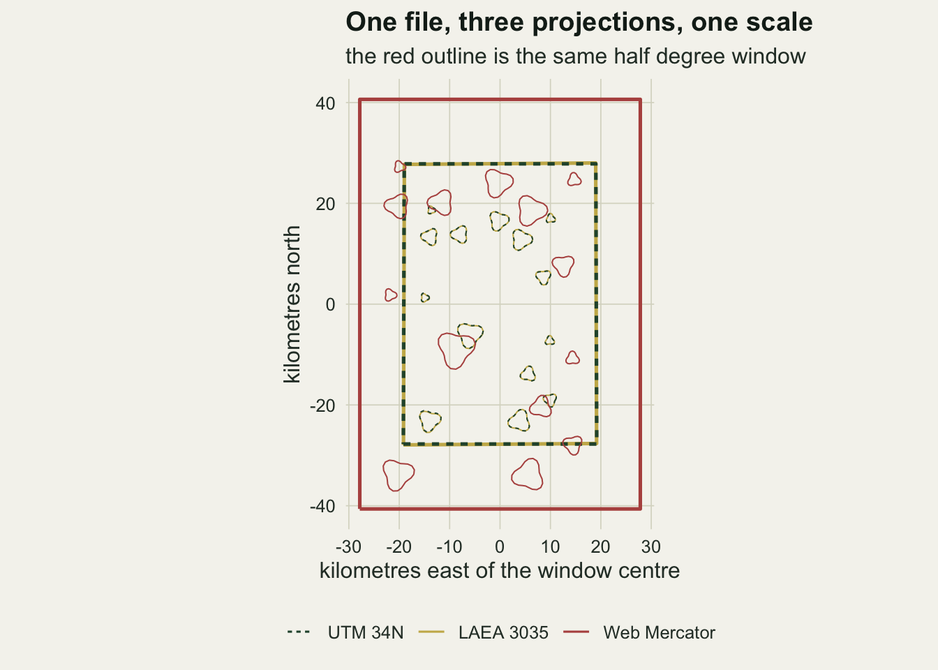
Web Mercator is a display projection. It exists so that tiles are square and north is up at every zoom level, and it is the correct choice for putting a basemap behind your data. It is never the right choice for a measurement, at any latitude away from the equator, and the error grows as you move away from it. Battersby and colleagues make the same separation from the cartographic side: the projection was adopted for tile serving, it was never intended to carry analysis, and the sphere it uses with ellipsoidal coordinates is not a defensible surface for measuring on.
Each outline in that figure has been turned so that true north points up, because otherwise the equal-area frame arrives visibly rotated: its origin is far to the west, and at this longitude its grid north sits 10.1 degrees off true north against 1.9 degrees for UTM. Rotation costs nothing in area or distance, but it is the first thing a reader notices when a layer is reprojected, and it is not evidence of a problem.
The gap between the two sensible projections is also a property of the extent rather than a general licence. Over half a degree the conformal and the equal-area answers differ by 0.017 per cent. Over 6 degrees on a side, as wide as a UTM zone but centred on the meridian where zone 34 hands over to zone 35, the difference is 0.11 per cent, with the conformal system running high because it is not built to hold area. The advice to use an equal-area projection for area is about extent: at a study site it changes almost nothing, and the gap widens as the extent does, which is why a continental reporting system such as EPSG:3035 exists and why UTM is not meant to be carried outside its own zone.
Two right answers disagree, and neither is broken
The s2 answer and the equal-area answer differ by 0.264 per cent, and a reader who sees that will assume one of them is wrong. Neither is. They are answers to two slightly different questions, and the difference can be predicted before either is computed.
s2 works on a sphere. The projections work on the WGS84 ellipsoid. The area of a lon/lat rectangle has a closed form on both surfaces, so both can be written out directly and compared.
d2r <- pi / 180
r_s2 <- 6371010                              # the sphere radius s2 uses, metres
a_ax <- 6378137; f_ell <- 1 / 298.257223563  # WGS84
e_sq <- f_ell * (2 - f_ell); e_ecc <- sqrt(e_sq)
sph_quad <- r_s2^2 * (2 * half * d2r) *
  (sin((lat0 + half) * d2r) - sin((lat0 - half) * d2r)) / 1e6

zone_area <- function(p) {                   # ellipsoidal area up to latitude p
  s <- sin(p * d2r)
  a_ax^2 * (1 - e_sq) * (s / (2 * (1 - e_sq * s^2)) +
    log((1 + e_ecc * s) / (1 - e_ecc * s)) / (4 * e_ecc))
}
ell_quad <- (2 * half * d2r) * (zone_area(lat0 + half) - zone_area(lat0 - half)) / 1e6
w_lat <- sqrt(1 - e_sq * sin(lat0 * d2r)^2)
rad_n <- a_ax / w_lat                        # prime vertical, east to west
rad_m <- a_ax * (1 - e_sq) / w_lat^3         # meridional, north to south
km_merid <- pi * rad_m / 180 / 1000          # one degree of latitude here
pred_area_pct <- 100 * ((sqrt(rad_m * rad_n) / r_s2)^2 - 1)
obs_area_pct  <- 100 * (win_area[3] / win_area[1] - 1)
The spherical rectangle is 2117.17 square kilometres and the ellipsoidal one is 2122.76. The s2 measurement lands within 0.0004 per cent of the spherical value and the equal-area projection lands within 0.0011 per cent of the ellipsoidal one. Each library is doing its own arithmetic correctly on its own surface.
The size of the gap follows from the curvature of the ellipsoid at this latitude. The radius of curvature is 6369 kilometres in the north to south direction and 6390 kilometres in the east to west direction, against s2’s single sphere of 6371. Area scales with the product of the two, which predicts a gap of 0.264 per cent against the 0.264 per cent measured. The meridional radius also fixes the length of a degree of latitude at this site, 111.166 kilometres. The rule of thumb multiplier used earlier, 111.32, is the equatorial degree of longitude, which is why it is a rule of thumb and not a measurement.
Distance is where this becomes interesting, because the two radii differ and a distance only feels one combination of them. A north to south line is measured against the meridional radius, an east to west line against the prime vertical, and everything else falls between. Sweeping the azimuth of a fixed length arm from the window centre and comparing s2 against a true ellipsoidal measurement shows the whole range.
aeqd <- sprintf("+proj=aeqd +lat_0=%.2f +lon_0=%.2f +datum=WGS84 +units=m +no_defs",
                lat0, lon0)
ctr <- st_sfc(st_point(c(lon0, lat0)), crs = 4326)
arm_m <- 40000; az_seq <- seq(0, 180, by = 5)
az_pct <- vapply(az_seq, function(a) {
  th  <- a * d2r
  far <- st_transform(
    st_sfc(st_point(c(arm_m * sin(th), arm_m * cos(th))), crs = aeqd), 4326)
  100 * (as.numeric(st_distance(c(ctr, far))[1, 2]) / arm_m - 1)
}, 0)
pred_ew <- 100 * (r_s2 / rad_n - 1)
pred_ns <- 100 * (r_s2 / rad_m - 1)
az_min  <- min(az_pct); az_max <- max(az_pct)
The azimuthal equidistant projection centred on the window measures true ellipsoidal distance from that centre, so the arm is 40 kilometres by construction and the deviation is entirely s2’s. It runs from -0.289 per cent at azimuth 90 degrees to 0.029 per cent at azimuth 180 degrees, against curvature predictions of -0.289 and 0.026 per cent. The sphere is too small for an east to west line here and very slightly too large for a north to south one.
az_df <- data.frame(az = az_seq, pct = az_pct)
ggplot(az_df, aes(az, pct)) +
  geom_hline(yintercept = c(pred_ew, pred_ns), linetype = "dashed",
             colour = te_rust, linewidth = 0.5) +
  geom_line(colour = te_forest, linewidth = 0.9) +
  geom_point(colour = te_ink, size = 1.6) +
  scale_x_continuous(breaks = seq(0, 180, by = 45)) +
  labs(x = "azimuth of the arm (degrees clockwise from north)", y = "s2 minus ellipsoid (per cent)",
       title = "The sphere is wrong by a different amount in each direction",
       subtitle = "dashed red: prediction from the two radii of curvature") +
  theme_datasheet()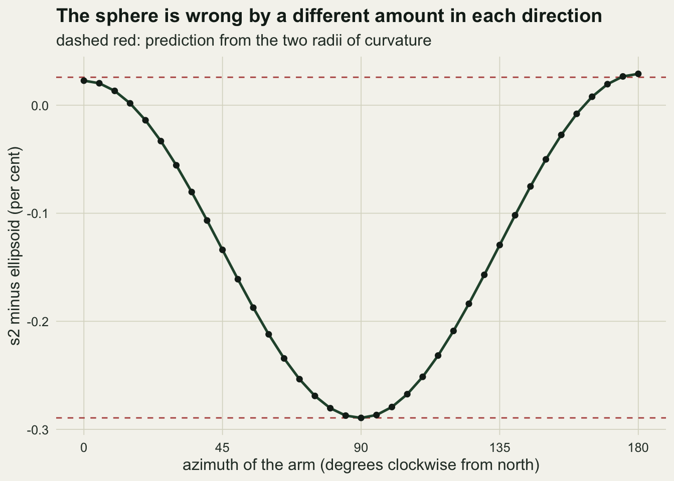
st_buffer returns a polygon, not a circle
A buffer is the second place where a measured area quietly loses a fixed percentage. st_buffer() on projected data returns a polygon whose vertices sit on the true circle, so the polygon is inscribed and its area is always short. For a regular polygon with n vertices inscribed in a circle of radius r, the area is n * r^2 * sin(2 * pi / n) / 2 against the circle’s pi * r^2, so the ratio is a closed form that depends only on n. sf takes its argument as segments per quadrant, so n is four times nQuadSegs.
ngon_ratio <- function(n) (n / (2 * pi)) * sin(2 * pi / n)
pt_utm <- st_sfc(st_point(as.numeric(st_coordinates(st_transform(ctr, 32634)))), crs = 32634)
buf_r <- 1000
seg_default <- eval(formals(sf::st_buffer)$nQuadSegs)   # what sf uses by default
seg_coarse  <- 5                                             # what several GUIs use
seg_seq <- c(2, 4, seg_coarse, 8, 12, seg_default, 60)
buf_tab <- data.frame(
  quad_seg = seg_seq, vertices = 4 * seg_seq,
  area_ratio = vapply(seg_seq, function(nq)
    as.numeric(st_area(st_buffer(pt_utm, buf_r, nQuadSegs = nq))) / (pi * buf_r^2), 0),
  closed_form = ngon_ratio(4 * seg_seq))
buf_tab$deficit_pct <- 100 * (1 - buf_tab$area_ratio)
max_err  <- max(abs(buf_tab$area_ratio - buf_tab$closed_form))
def_fine <- buf_tab$deficit_pct[match(seg_default, buf_tab$quad_seg)]
def_gui  <- buf_tab$deficit_pct[match(seg_coarse,  buf_tab$quad_seg)]
mant_thr <- 0.05 / (def_gui / 100)           # leading digits above this move a 2nd figure
knitr::kable(buf_tab, row.names = FALSE, digits = c(0, 0, 6, 6, 4),
caption = "Buffer area as a fraction of the circle it approximates.")| quad_seg | vertices | area_ratio | closed_form | deficit_pct |
|---|---|---|---|---|
| 2 | 8 | 0.900316 | 0.900316 | 9.9684 |
| 4 | 16 | 0.974495 | 0.974495 | 2.5505 |
| 5 | 20 | 0.983632 | 0.983632 | 1.6368 |
| 8 | 32 | 0.993587 | 0.993587 | 0.6413 |
| 12 | 48 | 0.997147 | 0.997147 | 0.2853 |
| 30 | 120 | 0.999543 | 0.999543 | 0.0457 |
| 60 | 240 | 0.999886 | 0.999886 | 0.0114 |
The measured ratios match the closed form to within floating-point rounding, so this is an identity and not an approximation. At sf’s default of 30 segments per quadrant the deficit is 0.046 per cent, which no ecological question will notice. At 5 segments per quadrant, which is the default in several GIS tools and in some older tutorials, it is 1.64 per cent. An error that size shifts the second significant figure of a home range or a foraging radius whenever the leading digits of the value sit above about 3.1, and only the third figure below that.
Buffering unprojected data is a different operation with a different failure. s2 does not build an inscribed polygon at all: it returns a covering assembled from S2 cells, nQuadSegs is ignored, and the controlling argument is max_cells.
circle_frac <- function(g) as.numeric(st_area(g)) / (pi * buf_r^2)
buf_ll <- st_buffer(ctr, buf_r); bb <- st_bbox(buf_ll)
ll_verts  <- nrow(st_coordinates(buf_ll)) - 1
ll_ratio  <- circle_frac(buf_ll)
ll_aspect <- as.numeric((bb[3] - bb[1]) / (bb[4] - bb[2]))
inv_cos   <- 1 / cos(lat0 * d2r)
ll_same   <- circle_frac(st_buffer(ctr, buf_r, nQuadSegs = seg_coarse))
mc_seq <- c(100, 1000, 5000, 20000)
mc_pct <- vapply(mc_seq,
  function(m) 100 * (circle_frac(st_buffer(ctr, buf_r, max_cells = m)) - 1), 0)
At the default the result carries 596 vertices and its area is 1.56 per cent above the circle, not below it, because a cell covering wraps the shape from outside. Asking for 5 segments per quadrant changes nothing: the area is still 1.56 per cent high. Dropping max_cells to 100 puts it 14.3 per cent high, and raising it to 20000 brings it down to 0.06 per cent. The bounding box is the visible tell: it is 1.47 times wider in degrees than it is tall, tracking one over the cosine of the latitude, 1.46.
The two errors point in opposite directions. A projected buffer is too small by a known amount you can set to nothing; a lon/lat buffer is too large by an amount that depends on a tiling argument most people have never seen.
mk_arc <- function(g, lab) {
  xy <- as.data.frame(st_coordinates(g)); data.frame(x = xy$X, y = xy$Y, kind = lab)
}
buf_at <- function(nq) st_buffer(st_sfc(st_point(c(0, 0)), crs = aeqd), buf_r, nQuadSegs = nq)
th_fine <- seq(0, 2 * pi, length.out = 2000)
arc_lab <- c("5 per quadrant", "30 per quadrant", "s2 cell covering", "true circle")
arcs <- rbind(
  mk_arc(buf_at(seg_coarse),  arc_lab[1]),
  mk_arc(buf_at(seg_default), arc_lab[2]),
  mk_arc(st_transform(buf_ll, aeqd), arc_lab[3]),
  data.frame(x = buf_r * sin(th_fine), y = buf_r * cos(th_fine), kind = arc_lab[4]))
arcs$kind <- factor(arcs$kind, levels = arc_lab)
p_arc <- ggplot(arcs, aes(x, y, colour = kind, linetype = kind)) +
  geom_path(linewidth = 0.7) +
  scale_colour_manual(values = c(te_gold, te_forest, te_rust, te_ink), name = NULL) +
  scale_linetype_manual(values = c("solid", "solid", "solid", "dashed"), name = NULL) +
  guides(colour = guide_legend(nrow = 2), linetype = guide_legend(nrow = 2)) +
  coord_cartesian(xlim = c(-300, 300), ylim = c(930, 1035)) +
  labs(x = "metres east of the centre", y = "metres north",
       title = "None of them is a circle") +
  theme_datasheet() +
  theme(legend.position = "bottom", legend.text = element_text(size = 8),
        legend.key.height = unit(0.8, "lines"))
curve_df <- data.frame(nq = seq(min(seg_seq), max(seg_seq), length.out = 400))
curve_df$pct <- 100 * (1 - ngon_ratio(4 * curve_df$nq))

p_def <- ggplot(curve_df, aes(nq, pct)) +
  geom_line(colour = te_forest, linewidth = 0.8) +
  geom_point(data = buf_tab, aes(quad_seg, deficit_pct), colour = te_ink, size = 2.2) +
  scale_y_log10() +
  labs(x = "nQuadSegs (segments per quadrant)", y = "area deficit (per cent, log scale)",
       title = "And the shortfall is exact",
       subtitle = "line: closed form; points: measured") +
  theme_datasheet()
p_arc + p_def + plot_annotation(theme = theme_datasheet())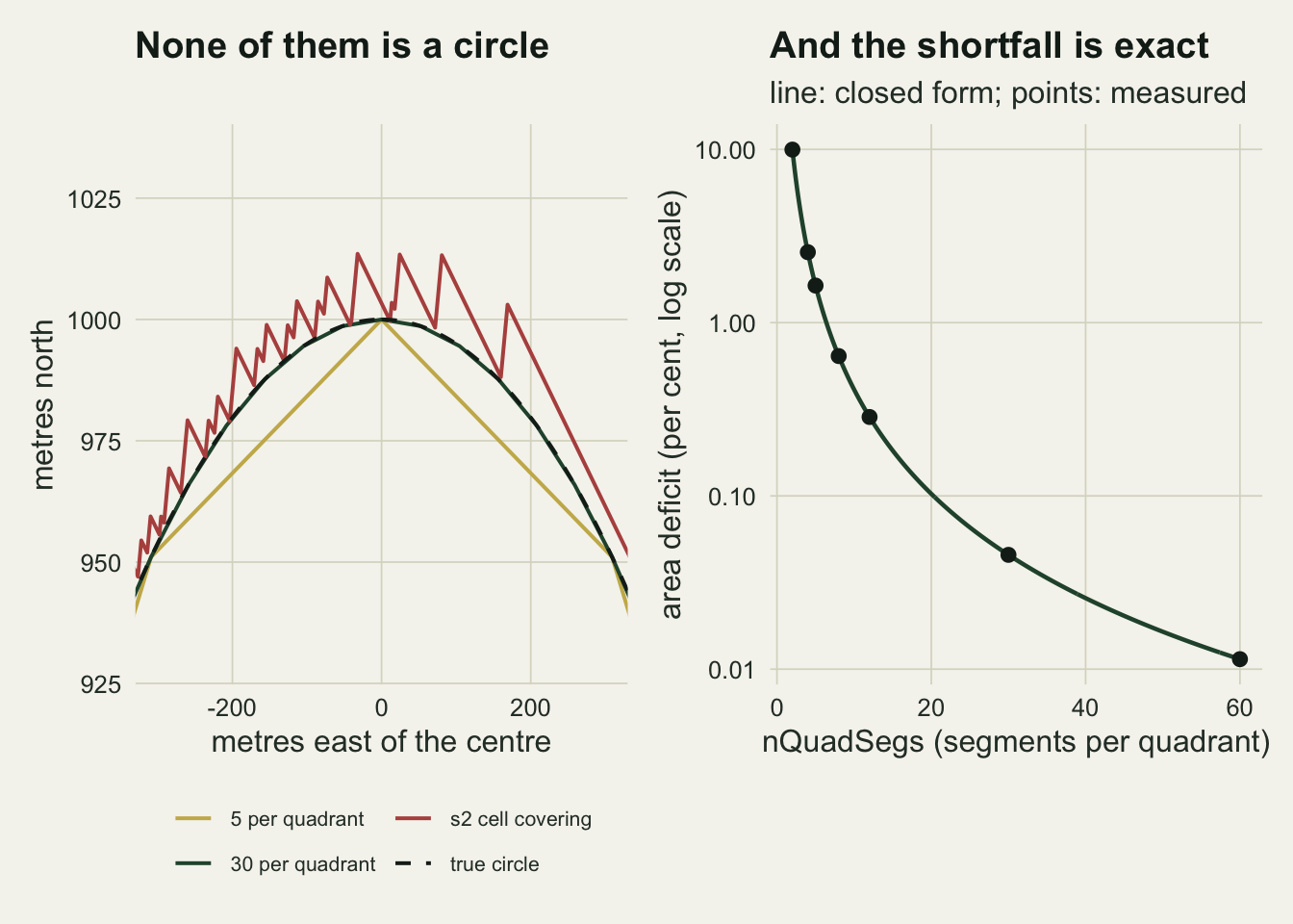
What it does to an ecological number
Back to the three quantities the survey wanted. Total habitat area, fragment density per hundred square kilometres, and the mean distance from a fragment to its nearest neighbour, each computed four times from the same file. Those three are ordinary fragmentation descriptors of the kind Fahrig separates into habitat loss and configuration effects, and the separation matters here because the two families answer to projection differently. Habitat cover as a percentage of the window is added as a fourth, because it is a ratio of two areas.
metrics_for <- function(e) {
  pp <- as_crs(patches_ll, e); ww <- as_crs(window_ll, e)
  ar <- as.numeric(st_area(pp)) / 1e6; wn <- as.numeric(st_area(ww)) / 1e6
  dm <- matrix(as.numeric(st_distance(pp)), n_patch) / 1000; diag(dm) <- NA
  c(habitat_km2 = sum(ar), cover_pct = 100 * sum(ar) / wn,
    density_100 = 100 * n_patch / wn,
    nn_km = mean(apply(dm, 1, min, na.rm = TRUE)))
}
eco_tab <- t(vapply(crs_code, metrics_for, numeric(4))); rownames(eco_tab) <- crs_lab
knitr::kable(eco_tab, digits = 3,
caption = "Four ecological quantities, one layer, four coordinate systems.")| habitat_km2 | cover_pct | density_100 | nn_km | |
|---|---|---|---|---|
| lon/lat, s2 | 98.403 | 4.648 | 0.661 | 4.919 |
| UTM 34N | 98.677 | 4.648 | 0.659 | 4.927 |
| LAEA 3035 | 98.663 | 4.648 | 0.660 | 4.920 |
| Web Mercator | 210.066 | 4.644 | 0.310 | 7.184 |
eco_dev <- 100 * (t(t(eco_tab) / eco_tab["UTM 34N", ]) - 1)
wm_dev  <- eco_dev["Web Mercator", ]; s2_dev <- eco_dev["lon/lat, s2", ]
Under Web Mercator the habitat area is 113 per cent high and the mean nearest neighbour distance is 46 per cent high, both of which anyone would catch. Fragment density is 53 per cent low, which is the same error wearing a different sign: the count is right and the denominator has more than doubled. That one is easy to miss in a table of results, and it is the number a fragmentation analysis usually reports.
Habitat cover survives. It comes back 0.077 per cent away from the UTM answer, because the numerator and the denominator are inflated by almost the same factor and the inflation cancels. The residual is not zero because Mercator’s scale factor changes with latitude across the window, so the fragments in the north are stretched slightly more than the ones in the south.
Leaving the data in lon/lat and letting s2 do the work is the other end of the range: habitat area 0.28 per cent low, density 0.28 per cent high, nearest neighbour distance 0.17 per cent low, cover 0.002 per cent off. Those are the sphere against ellipsoid differences from the previous section arriving in the results table, and they are smaller than the seed-to-seed variation of any real fragment map.
metric_lab <- c(habitat_km2 = "habitat area", cover_pct = "cover per cent",
                density_100 = "fragment density", nn_km = "nearest neighbour")
eco_alt  <- eco_dev[rownames(eco_dev) != "UTM 34N", , drop = FALSE]
eco_long <- data.frame(
  system = factor(rownames(eco_alt), c("Web Mercator", "lon/lat, s2", "LAEA 3035")),
  metric = factor(rep(metric_lab[colnames(eco_alt)], each = nrow(eco_alt)), metric_lab),
  pct = as.numeric(eco_alt))
ggplot(eco_long, aes(metric, pct, fill = system)) +
  geom_col(width = 0.65) +
  geom_hline(yintercept = 0, colour = te_body, linewidth = 0.3) +
  facet_wrap(~ system, scales = "free_y") +
  scale_fill_manual(values = c(te_rust, te_forest, te_gold), guide = "none") +
  labs(x = NULL, y = "deviation from the UTM answer (per cent)",
       title = "Which numbers survive the wrong projection",
       subtitle = "note the three vertical scales") +
  theme_datasheet() +
  theme(axis.text.x = element_text(angle = 30, hjust = 1),
        strip.text = element_text(face = "bold"))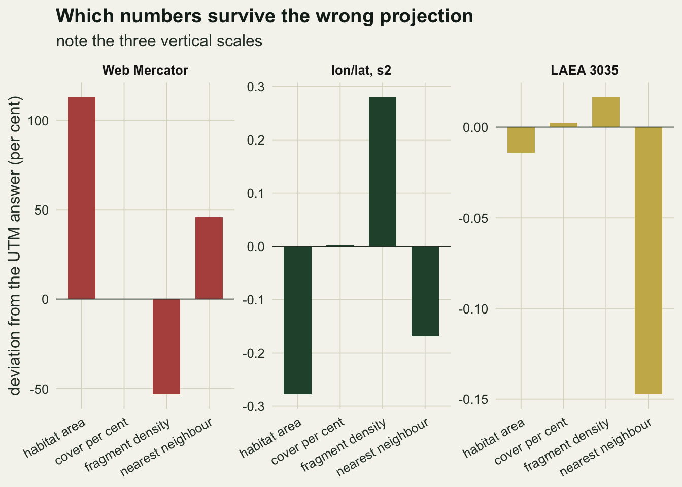
What to report
Give the EPSG code of the coordinate system every measurement was taken in, not just the one the data was stored in. Those are often different, and the transformation is where the number was decided.
For areas, use an equal-area projection appropriate to the extent. At a single study site the choice between a local conformal system and an equal-area one is worth hundredths of a per cent, and at the scale of a country it is worth tenths; either way the equal-area choice never costs anything, so there is no reason not to make it.
For distances, use a projection local to the extent, or skip the projection and let s2 measure the geodesic. Do not use an equal-area projection for distance work: it holds area by distorting shape, and the two baselines above show the mechanism, the east to west one coming out short of the conformal answer while the north to south one comes out long. At this extent each is off by a little over a tenth of a per cent, so the reason to keep the two jobs apart is the mechanism rather than the size of the error here. And never report a measurement taken in Web Mercator at all. If a figure is drawn over web tiles, the drawing can happen in EPSG:3857 while the numbers come from somewhere else; those are separate steps and only one of them is cartography.
If a buffer is anywhere in the pipeline, say what nQuadSegs or max_cells was, and say whether the buffer was built in projected or geographic coordinates. A percentage that appears in an abstract should not depend on an argument nobody wrote down.
Honest limits
The window here is 0.5 degrees on a side at 46.77 N. Everything scales with latitude: the Web Mercator inflation is one over the cosine of the latitude, so it is smaller in the tropics and far worse in the Arctic, and the sphere against ellipsoid gap changes sign and magnitude with latitude as well. The numbers in this post are the numbers at this latitude and this extent, not constants.
The edges of the window are not the same curve in every system. s2 joins the corners with great circle arcs, a projected system joins them with straight lines in its own plane, and those are different lines on the ground. At half a degree the difference is far below the effects measured here, but for a polygon spanning tens of degrees it is a real term and densifying the edges before transforming is the standard repair.
The azimuthal equidistant projection was treated as ground truth for distance. It holds distance exactly from its own centre, which is what the sweep uses it for, and PROJ’s ellipsoidal implementation is very accurate at the 40 kilometre range used here. It would not be a fair reference for longer arms, and a proper geodesic solver of the kind described by Karney is the right tool for those.
The fragments are synthetic, non-overlapping and convex enough that nearest neighbour distance between polygon edges is well behaved. Real fragment maps carry slivers, holes and topological errors, all of which change area and distance more than the choice of projection does. Checking a layer before measuring it is a separate job and it should come first.
Nothing here touches the datum either. Every system used is on WGS84 or ETRS89, and those two are not one frame: ETRS89 is pinned to the Eurasian plate while WGS84 follows ITRF, so they have been separating at roughly two and a half centimetres a year since the late nineteen eighties and are close to a metre apart in central Europe by now. Against a window tens of kilometres wide that shift is a few thousandths of a per cent, so the two are treated here as the same. Mixing a layer on an older national datum with one on WGS84 introduces shifts of tens or hundreds of metres, a larger error than anything measured above, and it is not fixed by choosing a better projection.
References
Pebesma E 2018 The R Journal 10(1):439-446 (10.32614/RJ-2018-009)
Pebesma E, Bivand R 2023 Spatial Data Science: With Applications in R (ISBN 978-0-429-45901-6)
Snyder JP 1987 US Geological Survey Professional Paper 1395 (10.3133/pp1395)
Karney CFF 2013 Journal of Geodesy 87(1):43-55 (10.1007/s00190-012-0578-z)
Battersby SE, Finn MP, Usery EL, Yamamoto KH 2014 Cartographica 49(2):85-101 (10.3138/carto.49.2.2313)
Fahrig L 2003 Annual Review of Ecology Evolution and Systematics 34(1):487-515 (10.1146/annurev.ecolsys.34.011802.132419)