library(ggplot2)
library(patchwork)
library(sf)

te_paper  <- "#f5f4ee"
te_ink    <- "#16241d"
te_body   <- "#2c3a31"
te_forest <- "#275139"
te_rust   <- "#b5534e"
te_gold   <- "#c9b458"
te_line   <- "#dad9ca"

theme_datasheet <- function() {
  theme_minimal(base_size = 12) +
    theme(plot.background  = element_rect(fill = te_paper, colour = NA),
          panel.background = element_rect(fill = te_paper, colour = NA),
          panel.grid.major = element_line(colour = te_line, linewidth = 0.3),
          panel.grid.minor = element_blank(),
          text             = element_text(colour = te_body),
          plot.title       = element_text(colour = te_ink, face = "bold"),
          plot.subtitle    = element_text(colour = te_body),
          axis.text        = element_text(colour = te_body))
}

geos_ver <- unname(sf::sf_extSoftVersion()["GEOS"])
gdal_ver <- unname(sf::sf_extSoftVersion()["GDAL"])Checking a vector layer before you measure
R
sf
GIS
spatial
ecology tutorial
A self-intersecting polygon has an area of exactly zero and sf says nothing. Eight geometry checks in R, each one measured on a synthetic habitat patch layer.
Updated 27 September 2026: a new section, The warning the overlay suppressed, explains what sf means by attributes assumed spatially constant and measures, on this block’s own records, how far summing a count over overlay pieces and area weighting miss the true count in a reserve.
A habitat map arrives as a GeoPackage: sixty patches of semi-natural grassland over a block ten kilometres on a side, digitised from aerial photographs across two field seasons, with occurrence records for a grassland butterfly to go with it. The first things anyone does with such a file are to measure it and to join to it: total habitat area, mean patch size, records per hectare, and a point in polygon join that tells each record which patch it sits in. Every one of those numbers comes back without a warning.
Six of the sixty patches carry a digitising slip, one vertex dragged out of order. Fifteen were traced twice, once in each field season, because the two seasons overlapped along a strip in the middle of the block. Nothing in the file records either fact. The slipped patches report between forty and fifty five per cent of the area they cover on the ground, the doubled ones are counted twice, and the join returns more rows than it was given. All of it is silent.
That is the difference between a broken vector layer and a broken table. A malformed CSV throws on read. An invalid polygon is not a corrupt file: it is a valid file describing an impossible shape, and every function downstream answers the question you asked as if the shape were fine. Cleaning GBIF and iNaturalist records handles the attributes of point records, the impossible latitudes and the null island coordinates; Mapping species richness in R with sf then measures. What sits between them is a check on the geometry itself. Joining ecological tables without losing zeros covers what a join does to a row count on the attribute side, where an inner join deletes the sites a species was absent from; the geometric version runs the other way, adding rows because two polygons cover the same ground.
Everything below is synthetic: the patches, the records and the two vegetation maps are built in the chunks, so each check ends with a truth to score against. Anything scored against that truth is a demonstration of a mechanism rather than a check you could run on a delivered file, and it is labelled as such where it appears. The answers depend on the geometry engine underneath sf, and that version is pulled from the session rather than typed.
The engine is GEOS 3.13.0 behind GDAL 3.8.5. Everything is in a projected system with metres for units (UTM zone 34 north, EPSG 32634), so the areas below are planar and the spherical geometry path is not involved.
A self-intersecting polygon has an area of exactly zero
The smallest possible case is a square whose corner coordinates were entered in the wrong order, so the ring crosses itself in the middle. It costs four vertices to reproduce, and it is worth reproducing at that size before it is run on sixty patches.
side_m   <- 30
bow_ring <- cbind(c(0, side_m, 0, side_m, 0), c(0, 0, side_m, side_m, 0))
bowtie   <- st_sfc(st_polygon(list(bow_ring)), crs = 32634)

bow_valid  <- st_is_valid(bowtie)
bow_reason <- st_is_valid(bowtie, reason = TRUE)
bow_area   <- as.numeric(st_area(bowtie))
sq_area    <- side_m^2
print(c(is_valid = bow_valid))
is_valid
FALSE print(bow_reason)[1] "Self-intersection[15 15]"print(c(area_m2 = bow_area, intended_square_m2 = sq_area)) area_m2 intended_square_m2
0 900 st_is_valid returns FALSE and gives the reason and the coordinates of the crossing. st_area returns 0 square metres against an intended 900, without a warning, a message or a note. The mechanism explains the whole post: the area of a ring is the signed shoelace sum over its edges, the two lobes of a crossed ring are traced in opposite directions, and their signed areas cancel exactly.
Three repairs are on offer and they do not agree.
fix_valid  <- st_make_valid(bowtie)
fix_buffer <- st_buffer(bowtie, 0)
fix_union  <- st_union(bowtie)

a_valid  <- as.numeric(st_area(fix_valid))
a_buffer <- as.numeric(st_area(fix_buffer))
a_union  <- as.numeric(st_area(fix_union))
buf_share <- a_buffer / a_valid

bow_class <- class(bowtie[[1]])[2]
uni_class <- class(fix_union[[1]])[2]
uni_valid <- st_is_valid(fix_union)
uni_same  <- identical(st_as_text(fix_union), st_as_text(bowtie))

probe   <- st_sfc(st_point(c(side_m / 2, side_m / 5)), crs = 32634)
in_lobe <- st_intersects(probe, bowtie, sparse = FALSE)[1, 1]
say <- function(expr) tryCatch({expr; "returned a result"},
                               error = function(e) "threw an error")
mute <- function(expr) {                  # did it warn or message on the way?
  loud <- FALSE
  withCallingHandlers(try(expr, silent = TRUE),
    warning = function(w) {loud <<- TRUE; invokeRestart("muffleWarning")},
    message = function(m) {loud <<- TRUE; invokeRestart("muffleMessage")})
  !loud
}
one_arg <- unique(c(say(st_make_valid(bowtie)), say(st_buffer(bowtie, 0)),
                    say(st_union(bowtie))))       # one word if all three agree
ovl_try <- say(st_intersection(bowtie, st_buffer(bowtie, 5)))
two_arg <- unique(c(ovl_try, say(st_union(bowtie, st_buffer(bowtie, 5)))))
quiet_of <- c(mute(st_make_valid(bowtie)), mute(st_buffer(bowtie, 0)),
              mute(st_union(bowtie)), mute(st_area(bowtie)),
              mute(st_intersects(probe, bowtie)))
n_quiet <- sum(quiet_of)

print(c(make_valid_m2 = a_valid, buffer_zero_m2 = a_buffer,
        unary_union_m2 = a_union))
make_valid_m2 buffer_zero_m2 unary_union_m2
450 225 0 print(c(union_type_in = bow_class, union_type_out = uni_class,
union_still_valid = uni_valid, union_wkt_unchanged = uni_same)) union_type_in union_type_out union_still_valid union_wkt_unchanged
"POLYGON" "POLYGON" "FALSE" "TRUE" print(c(point_in_polygon = in_lobe))point_in_polygon
TRUE print(c(one_geometry_in = one_arg, two_geometries_in = two_arg)) one_geometry_in two_geometries_in
"returned a result" "threw an error" print(c(calls_probed = length(quiet_of), raised_nothing = n_quiet)) calls_probed raised_nothing
5 5 st_make_valid returns a multipolygon of the two triangles the ring actually encloses, 450 square metres. st_buffer(x, 0), the older idiom still copied from forum answers, returns 225 square metres, a share of 0.50, because it keeps one lobe and discards the other. A unary st_union returns 0: it hands the ring straight back, class POLYGON in and POLYGON out, with well known text identical to the input, and st_is_valid on the result is still FALSE.
Two more results matter more than the repairs. A point inside one of the lobes tests as inside the polygon: st_intersects returns TRUE, so the join will find it. A polygon with no area still catches records, and a density of records per hectare in that polygon divides a positive count by zero. And an overlay of the bowtie against another polygon threw an error.
The line that splits these calls is not measurement against construction. st_make_valid, st_buffer(x, 0) and the unary st_union all construct new geometry, and all three returned a result, two of them something wrong. The calls that threw an error are the two that put the broken ring against a second geometry. Run those three constructions alongside st_area and st_intersects under a handler that catches warnings and messages and 0 of the 5 raise anything at all. The only operation that announces the problem is an overlay, and an overlay is not something anyone runs on read.
lab_bow <- c(sprintf("as digitised: st_area %.0f m2", bow_area),
             sprintf("st_make_valid: %.0f m2", a_valid),
             sprintf("st_buffer(x, 0): %.0f m2", a_buffer))
fac_bow  <- factor(lab_bow, levels = lab_bow)
mv_df    <- st_sf(panel = fac_bow[2], geometry = st_sfc(fix_valid, crs = 32634))
b0_df    <- st_sf(panel = fac_bow[3], geometry = st_sfc(fix_buffer, crs = 32634))
lost_df  <- st_sf(panel = fac_bow[3],
                  geometry = st_difference(st_geometry(mv_df), st_geometry(b0_df)))
node_df  <- data.frame(x = bow_ring[-5, 1] + c(-2.2, 2.2, -2.2, 2.2),   # each label
                       y = bow_ring[-5, 2] + c(-2.2, -2.2, 2.2, 2.2),   # outside its corner
                       lab = as.character(1:4), panel = fac_bow[1])

ggplot() +
  geom_sf(data = mv_df, fill = te_forest, colour = te_ink, linewidth = 0.4) +
  geom_sf(data = b0_df, fill = te_forest, colour = te_ink, linewidth = 0.4) +
  geom_sf(data = lost_df, fill = NA, colour = te_body, linewidth = 0.4,
          linetype = "22") +
  geom_path(data = data.frame(x = bow_ring[, 1], y = bow_ring[, 2],
                              panel = fac_bow[1]),
            aes(x, y), colour = te_ink, linewidth = 0.7) +
  geom_point(data = data.frame(x = side_m / 2, y = side_m / 2,
                               panel = fac_bow[1]),
             aes(x, y), shape = 21, size = 5, stroke = 1.2, colour = te_rust,
             fill = NA) +
  geom_text(data = node_df, aes(x, y, label = lab), colour = te_rust,
            size = 4) +
  facet_wrap(~panel) +
  coord_sf(xlim = side_m * c(-0.15, 1.15), ylim = side_m * c(-0.15, 1.15)) +
  labs(x = NULL, y = NULL, title = "Four corners in the wrong order") +
  theme_datasheet() +
  theme(axis.text = element_blank(), panel.grid = element_blank(),
        strip.text = element_text(colour = te_ink, face = "bold"),
        plot.margin = margin(8, 12, 8, 8))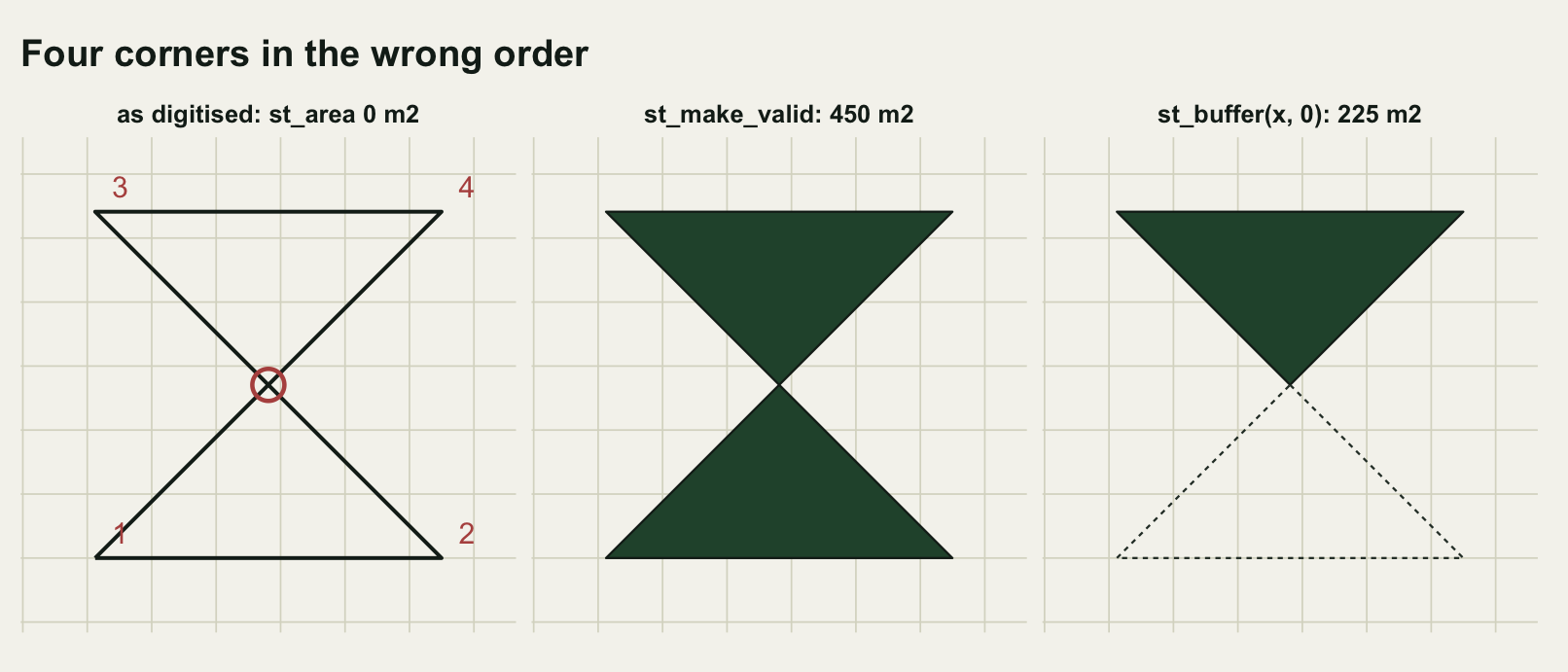
The same slip in a patch layer moves a density
Sixty grassland patches, no two of them touching, over a block ten kilometres on a side. The shapes are irregular blobs built from a smoothed radius around a centre, which is close enough to a digitised patch outline for the arithmetic to behave the same way.
ext_m <- 10000

mk_patch <- function(cx, cy, rad, nv = 16, rough = 0.16) {
  ang <- seq(0, 2 * pi, length.out = nv + 1)[-(nv + 1)]
  rr  <- rad * exp(rough * as.numeric(arima.sim(list(ar = 0.6), nv)))
  xy  <- cbind(cx + rr * cos(ang), cy + rr * sin(ang))
  st_polygon(list(rbind(xy, xy[1, ])))
}
set.seed(226101)
n_patch <- 60
cxv <- cyv <- rv <- numeric(0)
while (length(cxv) < n_patch) {                      # keep the patches apart
  r0 <- min(exp(rnorm(1, log(190), 0.5)), 600)
  xy0 <- runif(2, 1.8 * r0 + 100, ext_m - 1.8 * r0 - 100)
  if (!length(cxv) || min(sqrt((cxv - xy0[1])^2 + (cyv - xy0[2])^2) -
                          1.8 * (rv + r0)) > 100) {
    cxv <- c(cxv, xy0[1]); cyv <- c(cyv, xy0[2]); rv <- c(rv, r0)
  }
}
truth <- st_sf(patch_id = seq_len(n_patch),
               geometry = st_sfc(lapply(seq_len(n_patch), function(i)
                 mk_patch(cxv[i], cyv[i], rv[i])), crs = 32634))
a_true <- as.numeric(st_area(truth)) / 1e4
print(c(all_valid = all(st_is_valid(truth)),
        overlapping_pairs = sum(lengths(st_overlaps(truth)))))
all_valid overlapping_pairs
1 0 print(round(c(patches = n_patch, total_ha = sum(a_true), mean_ha = mean(a_true),
median_ha = median(a_true), largest_ha = max(a_true)), 3)) patches total_ha mean_ha median_ha largest_ha
60.000 787.544 13.126 9.070 94.302 The occurrence records are drawn at a constant intensity inside the habitat, so the expected density is the same in every patch. The realised counts are not: they are Poisson draws, a patch of a few hectares holds a handful of records, and the density a clean file reports swings widely from patch to patch before any geometry has gone wrong. That swing is the baseline any per-patch claim has to beat.
set.seed(226102)
n_cand   <- round(0.6 * ext_m^2 / 1e4)
cand_xy  <- cbind(runif(n_cand, 0, ext_m), runif(n_cand, 0, ext_m))
cand_pts <- st_sfc(lapply(seq_len(n_cand), function(i)
  st_point(cand_xy[i, ])), crs = 32634)
inside <- lengths(st_intersects(cand_pts, truth)) > 0
recs   <- st_sf(record_id = seq_len(sum(inside)), geometry = cand_pts[inside])
n_rec  <- nrow(recs)
dens_true <- n_rec / sum(a_true)
print(round(c(records = n_rec, true_density_per_ha = dens_true), 4))
records true_density_per_ha
494.0000 0.6273 Now the file as delivered. Six patches get a vertex slip, one vertex swapped with the vertex opposite it in the ring, which is what a mis-snapped drag produces. Fifteen, those in the strip surveyed in both seasons, appear a second time as an independent tracing of the same ground, vertices displaced by a couple of metres.
slip_ring <- function(p, k, d) {          # swap vertex k with the one opposite
  r <- p[[1]]; j <- (k + d - 1) %% (nrow(r) - 1) + 1
  r[c(k, j), ] <- r[c(j, k), ]; r[nrow(r), ] <- r[1, ]
  st_polygon(list(r))
}
wobble <- function(m, amp) {              # a repeatable per-vertex displacement
  d1 <- sin(0.9131 * m[, 1] + 1.2713 * m[, 2]) +
        sin(1.6421 * m[, 1] - 0.7331 * m[, 2])
  d2 <- sin(1.1877 * m[, 2] + 0.8419 * m[, 1]) +
        sin(0.7013 * m[, 2] - 1.4409 * m[, 1])
  cbind(m[, 1] + amp * d1 / sqrt(2), m[, 2] + amp * d2 / sqrt(2))
}
retrace <- function(p, amp) st_polygon(lapply(p, function(r) {
  o <- wobble(r, amp); o[nrow(o), ] <- o[1, ]; o }))

set.seed(226103)
slip_id <- sort(sample(n_patch, 6))
g_dig   <- st_geometry(truth)
set.seed(226104)
for (i in slip_id) g_dig[[i]] <- slip_ring(g_dig[[i]], sample(16, 1), 8)
ctr      <- st_coordinates(st_centroid(st_geometry(truth)))
twice_id <- which(ctr[, 1] >= 4000 & ctr[, 1] <= 6200)
g_two    <- st_sfc(lapply(twice_id, function(i)
  retrace(st_geometry(truth)[[i]], 4)), crs = 32634)
dig <- st_sf(season = c(rep("one", n_patch), rep("two", length(twice_id))),
             geometry = st_sfc(c(g_dig, g_two), crs = 32634))
dig$fid <- seq_len(nrow(dig))
n_feat  <- nrow(dig)
a_dig   <- as.numeric(st_area(dig)) / 1e4
print(c(features = n_feat, traced_twice = length(twice_id)))
features traced_twice
75 15 The validity scan is two lines and it is the whole of check one.
bad     <- !st_is_valid(dig)
n_bad   <- sum(bad)
a_fixed <- as.numeric(st_area(st_make_valid(dig))) / 1e4

slip_pct  <- 100 * a_dig[slip_id] / a_true[slip_id]
slip_gone <- sum(a_true[slip_id] - a_dig[slip_id])
slip_back <- sum(a_fixed[slip_id] - a_dig[slip_id])
slip_lost <- slip_gone - slip_back
tot_pct   <- 100 * (sum(a_dig) / sum(a_true) - 1)

print(c(invalid_features = n_bad))
invalid_features
6 print(round(cbind(patch = slip_id, true_ha = a_true[slip_id],
reported_ha = a_dig[slip_id],
repaired_ha = a_fixed[slip_id],
reported_pct_of_true = slip_pct), 3)) patch true_ha reported_ha repaired_ha reported_pct_of_true
[1,] 11 6.648 2.932 4.884 44.098
[2,] 32 13.291 5.349 9.354 40.243
[3,] 39 15.502 7.025 11.743 45.319
[4,] 46 2.934 1.277 2.206 43.507
[5,] 47 9.208 3.981 6.624 43.229
[6,] 57 12.148 6.626 9.605 54.545print(round(c(area_vanished_ha = slip_gone, recovered_by_repair_ha = slip_back,
unrecoverable_ha = slip_lost), 3)) area_vanished_ha recovered_by_repair_ha unrecoverable_ha
32.542 17.228 15.314 Each of the 6 slipped patches reports between 40.2 and 54.5 per cent of the area it covers on the ground. Together they take 32.5 hectares out of the layer’s total. st_make_valid puts 17.2 hectares of that back, and the remaining 15.3 hectares stay lost, because the repair recovers the two lobes the crossed ring actually encloses and not the patch the surveyor was tracing. That is the first thing to be clear about: st_make_valid gives you geometry you can measure, not the polygon somebody meant to draw.
The layer’s headline number does not show any of this, because the doubled patches push in the other direction.
join_all <- st_join(recs, dig, left = FALSE)
n_join   <- nrow(join_all)
join_pct <- 100 * (n_join / n_rec - 1)
rec_twice <- sum(table(join_all$record_id) > 1)
rec_lost  <- n_rec - length(unique(join_all$record_id))

rep_ha   <- sum(a_fixed)
union_ha <- as.numeric(st_area(st_union(st_make_valid(dig)))) / 1e4
twice_ha <- rep_ha - union_ha

print(round(c(true_total_ha = sum(a_true), reported_total_ha = sum(a_dig),
              inflation_pct = tot_pct,
              area_added_by_second_tracing_ha = sum(a_dig[(n_patch + 1):n_feat]),
              ground_covered_once_ha = union_ha,
              double_counted_ha = twice_ha), 3))
true_total_ha reported_total_ha
787.544 929.985
inflation_pct area_added_by_second_tracing_ha
18.087 174.983
ground_covered_once_ha double_counted_ha
779.275 167.938 print(c(records = n_rec, join_rows = n_join, matched_twice = rec_twice,
matched_never = rec_lost)) records join_rows matched_twice matched_never
494 599 111 6 The reported total is 930.0 hectares against a true 787.5, 18.1 per cent high, and the two errors that produced it have opposite signs: 32.5 hectares removed by the slips and 175.0 hectares added by the second tracing. A total is the statistic people sanity-check, and it is the statistic in which two large errors are most likely to hide each other.
The diagnostic that does see it costs one dissolve. Repairing the layer and taking the area of its union gives 779.3 hectares of ground covered at least once, against 947.2 hectares summed over the repaired features: 167.9 hectares are counted twice. Any layer whose feature sum and dissolved union disagree is not a partition of the ground, and every per-hectare quantity taken from the sum is wrong by their ratio.
The per-patch numbers need a baseline before they mean anything.
ok_id    <- setdiff(seq_len(n_patch), slip_id)
per_feat <- as.numeric(table(factor(join_all$fid, levels = seq_len(n_feat))))
dens_rep <- per_feat / a_dig
dens_med <- median(dens_rep)             # over every row, as a reader would take it

clean_rat <- dens_rep[ok_id] / dens_med  # what Poisson counts alone do
mean_cnt  <- mean(per_feat[ok_id])
n_zero    <- sum(per_feat[ok_id] == 0)

cnt_clean <- lengths(st_intersects(st_geometry(truth)[slip_id],
                                   st_geometry(recs)))
dens_cf   <- cnt_clean / a_true[slip_id]      # needs truth: not a field check
dens_slip <- per_feat[slip_id] / a_dig[slip_id]
slip_eff  <- dens_slip / dens_cf
slip_rat  <- dens_slip / dens_med
n_below   <- sum(clean_rat < min(slip_rat))
n_flag    <- sum(clean_rat >= min(slip_rat))  # cost of a cut that catches all six
n_over    <- sum(clean_rat > max(slip_rat))
hi_id     <- which.max(dens_rep)              # densest row in the delivered layer

lobe_share <- a_fixed[slip_id] / a_true[slip_id]
cnt_share  <- per_feat[slip_id] / cnt_clean
area_share <- a_dig[slip_id] / a_true[slip_id]

print(round(c(clean_patches = length(ok_id),
              mean_records_per_clean_patch = mean_cnt,
              clean_patches_with_no_records = n_zero,
              clean_ratio_to_median_min = min(clean_rat),
              clean_ratio_to_median_max = max(clean_rat)), 3))
clean_patches mean_records_per_clean_patch
54.000 8.370
clean_patches_with_no_records clean_ratio_to_median_min
3.000 0.000
clean_ratio_to_median_max
3.513 print(round(cbind(patch = slip_id, records_clean = cnt_clean,
records_as_slipped = per_feat[slip_id],
density_clean = dens_cf, density_as_slipped = dens_slip,
slip_effect = slip_eff, ratio_to_layer_median = slip_rat), 3)) patch records_clean records_as_slipped density_clean density_as_slipped
[1,] 11 5 4 0.752 1.364
[2,] 32 9 7 0.677 1.309
[3,] 39 15 11 0.968 1.566
[4,] 46 5 3 1.704 2.350
[5,] 47 4 3 0.434 0.754
[6,] 57 4 3 0.329 0.453
slip_effect ratio_to_layer_median
[1,] 1.814 2.188
[2,] 1.933 2.099
[3,] 1.618 2.511
[4,] 1.379 3.769
[5,] 1.735 1.209
[6,] 1.375 0.726print(round(c(slip_effect_min = min(slip_eff), slip_effect_max = max(slip_eff),
clean_below_lowest_slipped = n_below,
clean_flagged_with_all_six = n_flag,
clean_above_highest_slipped = n_over,
densest_row_in_layer = hi_id,
densest_row_is_slipped = hi_id %in% slip_id), 3)) slip_effect_min slip_effect_max
1.375 1.933
clean_below_lowest_slipped clean_flagged_with_all_six
15.000 39.000
clean_above_highest_slipped densest_row_in_layer
0.000 46.000
densest_row_is_slipped
1.000 Density is constant in expectation at 0.627 records per hectare and a clean patch holds 8.4 records on average, so the per-patch counts are small and Poisson. Take the median density over all 75 rows, which is the only median a reader has. The 54 clean patches run from 0.000 to 3.513 times it, 3 of them holding no records at all; the six slipped patches run 0.726 to 3.769. Those two ranges are not nested and they are not separated either. The densest row in the delivered layer is feature 46, one of the six, with 0 clean patches above it; but 15 clean patches sit below the lowest of the six, and a cut low enough to catch all six catches 39 of the 54 clean ones with them. Ranked against the layer median, a slip is counting noise.
What does separate them is not available in a delivered file. Score each slipped patch against its own clean counterfactual: join the records to the true outline of that patch and divide by its true area. That takes truth and a_true, and anyone holding those already knows which patches slipped, so read what follows as the mechanism rather than as a check. Against that counterfactual all six slipped patches read high, by 1.38 to 1.93 times, and none reads low, because the mechanism from the bowtie runs in one direction only. The crossed ring still encloses 70 to 79 per cent of the patch as two lobes and st_intersects answers for both, so the join keeps 60 to 80 per cent of the records, while st_area on the same ring reports 40 to 55 per cent of the true area, the two lobes being traced in opposite directions and partly cancelling. The numerator falls, the denominator falls further, and the density can only go up. 6 records match no feature at all.
Shao and Wu (2008) make the general point for landscape pattern work: area totals are the quantity least sensitive to data quality, and the metrics built on patch identity and patch size are the ones that move. A density is built on patch size.
lev_cls <- c("as digitised", "self-intersecting", "traced twice")
cls <- rep(lev_cls[1], n_feat)
cls[slip_id] <- lev_cls[2]
cls[(n_patch + 1):n_feat] <- lev_cls[3]
dig$class <- factor(cls, levels = lev_cls)
pal_edge <- setNames(c(te_forest, te_rust, te_gold), lev_cls)
pal_fill <- setNames(c("#cdd8cc", te_rust, te_gold), lev_cls)

p_map <- ggplot() +
  geom_sf(data = dig, aes(fill = class, colour = class), linewidth = 0.4,
          alpha = 0.9) +
  geom_point(data = as.data.frame(st_coordinates(recs)), aes(X, Y),
             inherit.aes = FALSE, colour = te_ink, size = 0.35, alpha = 0.6) +
  scale_fill_manual(values = pal_fill, name = NULL) +
  scale_colour_manual(values = pal_edge, name = NULL) +
  coord_sf(expand = FALSE) +
  guides(fill = guide_legend(nrow = 2), colour = guide_legend(nrow = 2)) +
  labs(x = NULL, y = NULL, title = "The layer as delivered") +
  theme_datasheet() +
  theme(legend.position = "bottom", axis.text = element_blank(),
        panel.grid = element_blank(), plot.margin = margin(8, 10, 8, 8))

p_sc <- ggplot(data.frame(true_ha = c(a_true, a_true[twice_id]),
                          rep_ha = a_dig, class = dig$class),
               aes(true_ha, rep_ha, colour = class)) +
  geom_abline(slope = 1, intercept = 0, linetype = "22", colour = te_ink,
              linewidth = 0.5) +
  geom_point(size = 2.1, alpha = 0.9) +
  scale_colour_manual(values = pal_edge, guide = "none") +
  scale_x_log10() + scale_y_log10() +
  labs(x = "true area (hectares)", y = "reported area (hectares)",
       title = "What each feature reports") +
  theme_datasheet() +
  theme(plot.margin = margin(8, 12, 8, 8))

p_map + p_sc + plot_annotation(theme = theme_datasheet())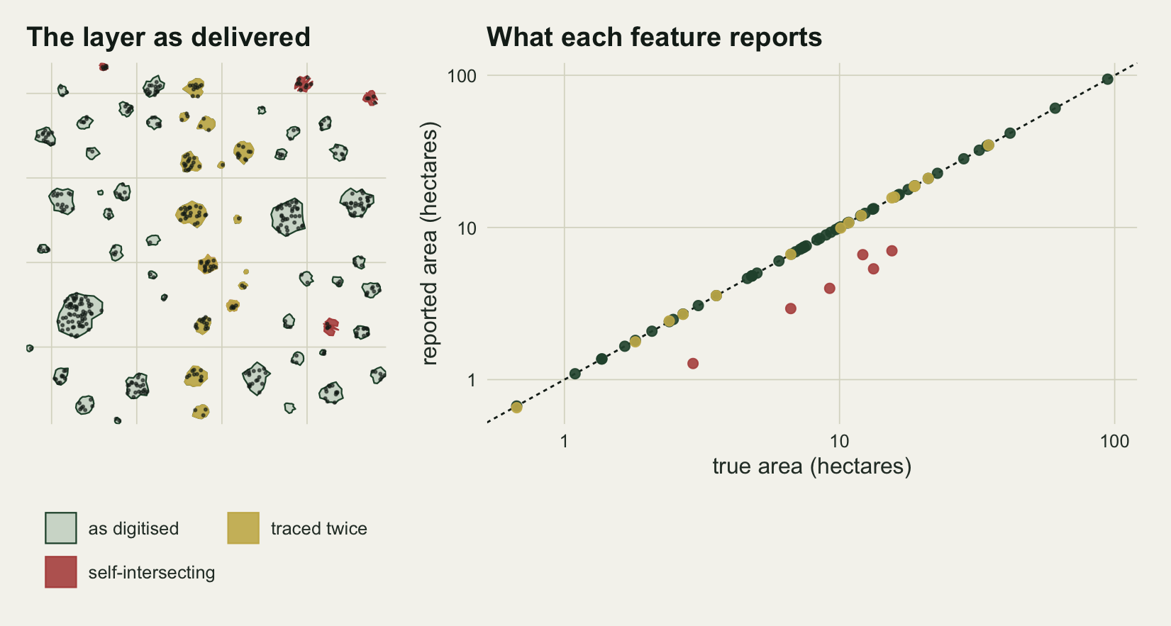
Most of the polygons in an overlay are not real
The second layer in the project is a vegetation map of the same block, twelve units tiling it completely, with a second edition made five years later. Between the editions one clearing was felled, six hectares of it, and nothing else changed. Everything else that differs between the files is two tracings of one boundary: the vertices sit fifty metres apart and the second edition displaces each one by an amount that depends on where it is, so the two boundaries wander across each other rather than sitting a fixed distance apart. Goodchild and Hunter (1997) formalise that wandering as a band of uncertainty around a digitised line, and the width of the band sets everything below.
block <- st_sfc(st_polygon(list(cbind(c(0, ext_m, ext_m, 0, 0),
                                      c(0, 0, ext_m, ext_m, 0)))), crs = 32634)
set.seed(226110)
n_unit <- 12
seeds  <- st_sfc(lapply(seq_len(n_unit), function(i)
  st_point(runif(2, 400, ext_m - 400))), crs = 32634)
vor <- st_collection_extract(st_voronoi(st_combine(seeds), envelope = block),
                             "POLYGON")
map_a <- st_sf(unit_a = seq_along(vor), geometry = st_segmentize(
  st_intersection(st_sfc(vor, crs = 32634), block), dfMaxLength = 50))

wob_amp <- 3
g_b     <- st_sfc(lapply(st_geometry(map_a), retrace, amp = wob_amp), crs = 32634)
node1   <- st_geometry(map_a)[[2]][[1]]
moved   <- wobble(node1, wob_amp)
move_m  <- sqrt(rowSums((moved - node1)^2))
gap_m   <- as.numeric(st_distance(
  st_sfc(lapply(seq_len(nrow(node1) - 1L), function(i) st_point(moved[i, ])),
         crs = 32634),
  st_cast(st_geometry(map_a)[2], "MULTILINESTRING")))

big_id <- which.max(as.numeric(st_area(map_a)))
cc     <- st_coordinates(st_centroid(st_geometry(map_a)[big_id]))
felled <- st_sfc(st_polygon(list(cbind(cc[1] + c(-150, 150, 150, -150, -150),
                                       cc[2] + c(-100, -100, 100, 100, -100)))),
                 crs = 32634)
fell_ha  <- as.numeric(st_area(felled)) / 1e4
other_id <- if (big_id == 1) 2 else 1
g_b[big_id]   <- st_difference(g_b[big_id], felled)
g_b[other_id] <- st_union(g_b[other_id], felled)
map_b <- st_sf(unit_b = seq_len(n_unit), geometry = g_b)

print(round(c(units = n_unit, mean_vertex_move_m = mean(move_m),
              max_vertex_move_m = max(move_m),
              mean_gap_between_boundaries_m = mean(gap_m),
              max_gap_between_boundaries_m = max(gap_m),
              real_change_ha = fell_ha), 3))
units mean_vertex_move_m
12.000 2.757
max_vertex_move_m mean_gap_between_boundaries_m
5.881 1.743
max_gap_between_boundaries_m real_change_ha
4.860 6.000 print(c(map_a_valid = all(st_is_valid(map_a)),
map_b_valid = all(st_is_valid(map_b))))map_a_valid map_b_valid
TRUE TRUE Both maps are valid, both tile the block, and the only real change between them is one polygon of 6 hectares. The change map is one st_intersection away.
ov <- suppressWarnings(st_intersection(map_a, map_b))
ov <- ov[st_geometry_type(ov) %in% c("POLYGON", "MULTIPOLYGON"), ]
pieces <- suppressWarnings(st_cast(st_cast(ov, "MULTIPOLYGON"), "POLYGON"))
pieces$area_m2 <- as.numeric(st_area(pieces))
chg <- pieces[pieces$unit_a != pieces$unit_b, ]

n_chg    <- nrow(chg)
chg_ha   <- sum(chg$area_m2) / 1e4
by_size  <- sort(chg$area_m2, decreasing = TRUE)
real_m2  <- by_size[1]
sliver_max <- by_size[2]
sliver_med <- median(by_size[-1])

print(c(overlay_rows = nrow(ov), individual_polygons = nrow(pieces),
        change_polygons = n_chg))
overlay_rows individual_polygons change_polygons
60 576 564 print(round(c(reported_change_ha = chg_ha, true_change_ha = fell_ha,
area_ratio = chg_ha / fell_ha,
largest_change_m2 = real_m2, largest_sliver_m2 = sliver_max,
median_sliver_m2 = sliver_med), 3))reported_change_ha true_change_ha area_ratio largest_change_m2
13.406 6.000 2.234 60000.000
largest_sliver_m2 median_sliver_m2
989.371 95.892 The overlay says 564 polygons changed vegetation class, covering 13.41 hectares. One polygon changed, covering 6 hectares. The count is wrong by a factor of 564 and the area by a factor of 2.23, and both numbers rest on real geometry: every sliver is a valid, positive-area polygon marking a place where the two files disagree. MacDougall (1975) worked this out for hand-drawn overlays half a century ago, and the arithmetic has not changed because it is a property of the boundaries, not of the software.
Note the first line of that output. The overlay has 60 rows and 576 polygons, because st_intersection returns one row per pair of input features and packs the pieces of each pair into a multipolygon. Counting patches with nrow() on the result of an overlay is the second silent failure in this section, and it happens to under-count rather than over-count.
Three repairs, and they cost different things.
thr_grid <- c(100, 500, 1100, 2000)
thr_tab  <- t(sapply(thr_grid, function(t0) {
  k <- chg[chg$area_m2 >= t0, ]
  c(threshold_m2 = t0, polygons = nrow(k), area_ha = sum(k$area_m2) / 1e4)
}))

tol_grid <- c(0.25, 0.5, 1, 1.5, 2, 5)
snap_tab <- t(sapply(tol_grid, function(tol) {
  snapped <- st_sf(unit_b = map_b$unit_b,
                   geometry = st_snap(st_geometry(map_b), st_geometry(map_a),
                                      tolerance = tol))
  o2 <- suppressWarnings(st_intersection(map_a, snapped))
  o2 <- o2[st_geometry_type(o2) %in% c("POLYGON", "MULTIPOLYGON"), ]
  p2 <- suppressWarnings(st_cast(st_cast(o2, "MULTIPOLYGON"), "POLYGON"))
  p2$area_m2 <- as.numeric(st_area(p2))
  c2 <- p2[p2$unit_a != p2$unit_b, ]
  c(tolerance_m = tol, still_valid = all(st_is_valid(snapped)),
    change_polygons = nrow(c2), change_ha = sum(c2$area_m2) / 1e4)
}))
i_work    <- which(snap_tab[, "change_polygons"] == 1)[1]
snap_work <- snap_tab[i_work, ]                 # first tolerance that gets it right
snap_near <- snap_tab[i_work - 1, ]             # the last one that does not
snap_lo   <- snap_tab[1, ]
gap_under <- mean(gap_m <= snap_work["tolerance_m"])

erode_tab <- t(sapply(c(2, 5, 10), function(bw) {
  bb <- suppressWarnings(st_buffer(st_buffer(st_union(st_geometry(chg)), -bw), bw))
  c(width_m = bw, parts = length(suppressWarnings(st_cast(st_sfc(bb), "POLYGON"))),
    area_ha = as.numeric(st_area(bb)) / 1e4)
}))

print(round(thr_tab, 4))
threshold_m2 polygons area_ha
[1,] 100 273 12.1799
[2,] 500 19 7.2419
[3,] 1100 1 6.0000
[4,] 2000 1 6.0000print(round(snap_tab, 4)) tolerance_m still_valid change_polygons change_ha
[1,] 0.25 1 250 9.0101
[2,] 0.50 1 105 7.4091
[3,] 1.00 1 20 6.1571
[4,] 1.50 1 3 6.0310
[5,] 2.00 1 1 6.0000
[6,] 5.00 1 1 6.0000print(round(c(working_tolerance_m = unname(snap_work["tolerance_m"]),
share_of_gaps_under_it = gap_under), 4)) working_tolerance_m share_of_gaps_under_it
2.0000 0.5856 print(round(erode_tab, 4)) width_m parts area_ha
[1,] 2 47 6.3353
[2,] 5 1 5.9979
[3,] 10 1 5.9914An area threshold works, and the measurement says exactly where it has to sit. The largest sliver is 989 square metres, so any threshold between that and the size of the change itself recovers the one real change and its 6.00 hectares exactly. That is also the cost: with vertices this far apart, no genuine change smaller than 0.10 hectares can be told from digitising disagreement, whatever threshold is chosen. The minimum mappable change is a property of the two files, and it is worth computing before the change map is drawn.
Snapping the second map onto the first before the overlay is the better repair when the second map can be edited, because it removes the slivers instead of filtering them. The count falls steeply with the tolerance: 250 change polygons at 0.25 metres, 3 at 1.50, and at 2.00 metres the overlay returns 1 change polygon of 6.00 hectares, which is the truth exactly. That working value is not read off the boundary statistics: it sits above the mean perpendicular gap of 1.74 metres and well under the largest gap of 4.86, and it covers 59 per cent of the sampled gaps rather than all of them. The gap distribution brackets the tolerance; the grid finds it. It must also stay under the smallest real feature, and if both conditions cannot be met the overlay cannot answer the question.
Eroding and dilating the change layer is the crudest of the three and it shows: at 2 metres it leaves 47 parts, and at 5 metres it returns one part of 5.9979 hectares, which has lost 0.0021 hectares to its own rounded corners. It is the option to reach for when the second layer cannot be edited.
half_w  <- 90
edge_pt <- st_coordinates(st_centroid(st_geometry(
  chg[order(chg$area_m2, decreasing = TRUE)[2], ])))
win <- st_sfc(st_polygon(list(cbind(
  edge_pt[1] + half_w * c(-1, 1, 1, -1, -1),
  edge_pt[2] + half_w * c(-1, -1, 1, 1, -1)))), crs = 32634)
line_a <- st_intersection(st_cast(st_geometry(map_a), "MULTILINESTRING"), win)
line_b <- st_intersection(st_cast(st_geometry(map_b), "MULTILINESTRING"), win)
line_b <- line_b[1]   # both neighbours trace the shared edge; draw it once so the dashes show
chg_win <- st_intersection(st_geometry(chg), win)

p_zoom <- ggplot() +
  geom_sf(data = chg_win, fill = te_rust, colour = te_rust, linewidth = 0.3) +
  geom_sf(data = line_a, colour = te_forest, linewidth = 0.7) +
  geom_sf(data = line_b, colour = te_ink, linewidth = 0.7, linetype = "22") +
  coord_sf(expand = FALSE) +
  labs(x = NULL, y = NULL, title = "Two tracings of one boundary",
       subtitle = "green solid: first edition; dark dashed: second") +
  theme_datasheet() +
  theme(axis.text = element_blank(), panel.grid = element_blank(),
        plot.margin = margin(8, 10, 8, 8))

p_hist <- ggplot(data.frame(a = chg$area_m2), aes(a)) +
  geom_histogram(bins = 34, fill = te_forest, colour = te_paper,
                 linewidth = 0.2) +
  geom_vline(xintercept = sliver_max, colour = te_rust, linetype = "22",
             linewidth = 0.7) +
  geom_vline(xintercept = real_m2, colour = te_gold, linewidth = 1.1) +
  scale_x_log10(breaks = 10^seq(-1, 5, by = 2),
                labels = function(v) format(v, scientific = FALSE,
                                            trim = TRUE, drop0trailing = TRUE)) +
  labs(x = "area of a change polygon (square metres)", y = "polygons",
       title = "One of these is a real change",
       subtitle = "dashed rust: largest sliver; gold: the felled block") +
  theme_datasheet() +
  theme(plot.margin = margin(8, 12, 8, 8))

p_zoom + p_hist + plot_annotation(theme = theme_datasheet())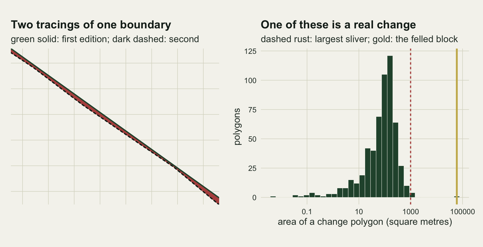
The warning the overlay suppressed
The overlay chunk wraps st_intersection(map_a, map_b) in suppressWarnings(). The chunk below runs the same call bare, then puts the block’s records into an atlas of two kilometre squares, the kind of grid layer Mapping species richness in R with sf builds, and draws a reserve over it: an irregular seven-sided polygon, the same shape at every placement, with its centre drawn at random in the middle four kilometres of the block so that it always lies inside it.
catch_warn <- function(expr) {                 # keep warnings as text
  said  <- character(0)
  value <- withCallingHandlers(expr, warning = function(w) {
    said <<- c(said, conditionMessage(w)); invokeRestart("muffleWarning")})
  list(value = value, said = said)
}
ov_run  <- catch_warn(st_intersection(map_a, map_b))
agr_run <- catch_warn(st_intersection(st_set_agr(map_a, "constant"),
                                      st_set_agr(map_b, "constant")))
map_a_n <- st_set_agr(map_a, "constant"); map_a_n$count <- 1   # added later
add_run <- catch_warn(st_intersection(map_a_n, st_set_agr(map_b, "constant")))
atlas <- st_sf(square = 1:25, geometry = st_make_grid(block, cellsize = 2000))
atlas$records <- lengths(st_intersects(st_geometry(atlas), st_geometry(recs)))
hab_sq <- st_set_agr(st_intersection(st_set_agr(atlas["square"], "constant"),
  st_union(st_make_valid(st_geometry(dig)))), "constant")  # an id is constant
hab_m2 <- replace(numeric(25), hab_sq$square, as.numeric(st_area(hab_sq)))
patch_share <- sum(a_true) / (ext_m^2 / 1e4)   # true patches: they do not overlap
mk_reserve <- function(cx, cy, k = c(1, 0.8, 1.1, 0.9, 1, 0.7, 1.05)) {
  ang <- seq(0, 2 * pi, length.out = 8)[-8]
  xy  <- cbind(cx + 1560 * k * cos(ang), cy + 1260 * k * sin(ang))
  st_sfc(st_polygon(list(xy[c(1:7, 1), ])), crs = 32634)
}
three_ways <- function(res) {
  pc <- catch_warn(st_intersection(atlas, res))
  aw <- catch_warn(st_interpolate_aw(atlas["records"], res, extensive = TRUE))
  hr <- st_intersection(hab_sq, res)
  sq <- pc$value$square
  c(truth = lengths(st_intersects(res, recs)), touched = length(sq),
    summed = sum(pc$value$records), area_wt = sum(aw$value$records),
    by_hand = sum(atlas$records[sq] * as.numeric(st_area(pc$value)) /
                  as.numeric(st_area(atlas))[sq]),
    dasymetric = sum(atlas$records[hr$square] * as.numeric(st_area(hr)) /
                     hab_m2[hr$square]),
    full_count_copied = all(pc$value$records == atlas$records[sq]))
}
res_ha  <- as.numeric(st_area(mk_reserve(5000, 5000))) / 1e4
one_res <- three_ways(mk_reserve(5000, 5000))
set.seed(226120)
n_place  <- 30
res_ctr  <- cbind(runif(n_place, 3000, 7000), runif(n_place, 3000, 7000))
many_res <- t(apply(res_ctr, 1, function(p) three_ways(mk_reserve(p[1], p[2]))))
sum_rat  <- many_res[, "summed"] / many_res[, "truth"]
rel_err  <- abs(many_res[, c("area_wt", "dasymetric")] / many_res[, "truth"] - 1)
whole_aw <- catch_warn(st_interpolate_aw(atlas["records"], block, extensive = TRUE))
has_wts  <- "weights" %in% names(formals(getS3method("st_interpolate_aw", "sf")))
stopifnot(length(ov_run$said) >= 1, length(add_run$said) >= 1,
          length(agr_run$said) == 0, length(whole_aw$said) >= 1,
          all(many_res[, "full_count_copied"] == 1),
          all(many_res[, "summed"] >= many_res[, "truth"]),
          all(abs(many_res[, "area_wt"] - many_res[, "by_hand"]) < 1e-6),
          abs(sum(whole_aw$value$records) - sum(atlas$records)) < 1e-6,
          has_wts == (packageVersion("sf") >= "1.1-1"))
print(c(ov_run$said, whole_aw$said))
[1] "attribute variables are assumed to be spatially constant throughout all geometries"
[2] "st_interpolate_aw assumes attributes are constant or uniform over areas of x" print(round(c(one_res[1:6], patch_share_of_block = patch_share), 3)) truth touched summed
39.000 6.000 133.000
area_wt by_hand dasymetric
41.118 41.118 40.615
patch_share_of_block
0.079 print(round(t(sapply(list(summed_over_truth = sum_rat, area_wt_rel_err = rel_err[, 1],
dasymetric_rel_err = rel_err[, 2]), quantile, probs = c(0, 0.5, 1))), 3)) 0% 50% 100%
summed_over_truth 2.278 4.500 15.000
area_wt_rel_err 0.003 0.263 2.107
dasymetric_rel_err 0.006 0.077 0.238i_worst <- which.max(rel_err[, 1]) # worst area-weighted placementRun bare, the overlay under sf 1.1-1 raises 1 warning: “attribute variables are assumed to be spatially constant throughout all geometries”. An overlay cuts each feature into pieces and copies the feature’s attributes onto every piece unchanged, and the warning is sf saying so. It cannot tell a column that holds at every point of a feature, such as a vegetation class, from one that is a total over the feature, such as a count, which a piece holds only part of. For unit_a and unit_b the copy is right, and saying so removes the warning: with both maps set to st_set_agr(x, "constant") the same overlay raises 0 warnings. The declaration belongs to the columns it names: a count column added to map_a afterwards carries none, and the overlay raises 1 warning again, which a suppressWarnings() would have silenced with the rest. For a count the copy is wrong.
The reserve at the centre of the block covers 465 hectares, touches 6 squares and holds 39 records. Summing records over its overlay pieces gives 133, because every touched square brings its full count however little of it lies inside. That overcount is arithmetic: the sum is the total of every square the reserve touches, so it can never fall below the truth, and the chunk checks that at every placement. Its size is set by how many records the touched squares hold outside the reserve, and over the 30 placements it runs from 2.3 to 15.0 times the true count.
st_interpolate_aw(extensive = TRUE) is the call built for a count. It gives each piece the share of its square’s count that matches the share of the square’s area it covers; over the whole block it returns the atlas total exactly, and the chunk checks it against the same shares computed by hand. It raises its own warning, “st_interpolate_aw assumes attributes are constant or uniform over areas of x”, which names its assumption. For the central reserve it gives 41.1 records, and across the placements its relative error has a median of 0.26 and a worst case of 2.11, at a placement holding 5 records. The records break the assumption by construction: they sit only in the grassland patches, which cover 7.9 per cent of the block, so a reserve boundary that cuts a square need not cut its records in the share it cuts its area. Weighting by each square’s habitat inside the reserve instead of its area (dasymetric mapping, here with the repaired delivered patch layer as the mask) brings the median relative error to 0.08 and is the closer of the two at 26 of the 30 placements; the placements overlap one another, so they show a spread, not independent trials. sf from 1.1-1 has an experimental weights argument to st_interpolate_aw() for dasymetric mapping, and it is not a drop-in for this: the weights are a column of the target layer, and each square’s count is shared only among the target pieces that square touches. Checked outside this post, by running the dasymetric() code of sf 1.1-3 on this atlas and the central reserve, the reserve alone as the target, weighted by its habitat area, got back the 133 records of the summed pieces, because every touched square hands its full count to its one piece; a target of two features, the habitat inside the reserve and the habitat outside it, each weighted by its area, gave the chunk’s 40.6. The chunk does it by hand so that it runs on either side of that version. Those two error sizes belong to this layout, not to the methods: one set of records, one grid, one reserve shape, and a mask that is, apart from the six slipped patches and the couple of metres by which the second tracings wander, the very layer the records were drawn inside, which no ancillary layer in real work will be. How the choice of zones can reverse the sign of a relationship is a different problem, taken up in When redrawing zones flips the sign.
Ring direction is not the problem: nested shells and empty rows are
Three smaller failures are worth a measurement each, and the first turns out not to be a failure in this stack at all. The simple features standard asks for an anticlockwise exterior ring and clockwise interior rings, GIS folklore treats a reversed ring as a source of negative areas, and sf on GEOS does not care.
rev_ring  <- function(p) st_polygon(list(p[[1]][nrow(p[[1]]):1, ]))
flipped   <- st_sfc(lapply(st_geometry(truth), rev_ring), crs = 32634)
ring_gap  <- max(abs(as.numeric(st_area(flipped)) - as.numeric(st_area(truth))))

k_big  <- which.max(a_true)
shell  <- st_geometry(truth)[[k_big]][[1]]
cen    <- colMeans(shell[-nrow(shell), ])
inner  <- cbind(cen[1] + 0.45 * (shell[, 1] - cen[1]),
                cen[2] + 0.45 * (shell[, 2] - cen[2]))
donut  <- st_sfc(st_polygon(list(shell, inner[nrow(inner):1, ])), crs = 32634)
nested <- st_sfc(st_multipolygon(list(list(shell), list(inner))), crs = 32634)

a_donut <- as.numeric(st_area(donut)) / 1e4
a_nest  <- as.numeric(st_area(nested)) / 1e4
a_nfix  <- as.numeric(st_area(st_make_valid(nested))) / 1e4

print(c(ring_direction_max_area_gap_m2 = ring_gap))
ring_direction_max_area_gap_m2
8.731149e-10 print(c(flipped_all_valid = all(st_is_valid(flipped))))flipped_all_valid
TRUE print(c(nested_is_valid = st_is_valid(nested)))nested_is_valid
FALSE print(st_is_valid(nested, reason = TRUE))[1] "Nested shells[1951.28178461081 3100.82416372762]"print(round(c(as_interior_ring_ha = a_donut, as_second_shell_ha = a_nest,
ratio = a_nest / a_donut, after_make_valid_ha = a_nfix), 3))as_interior_ring_ha as_second_shell_ha ratio after_make_valid_ha
75.206 113.398 1.508 94.302 Reversing every ring in the layer leaves every area the same to within floating-point rounding (the largest gap, printed above, is a tiny fraction of a square metre), and every reversed polygon is still valid. Winding order is not a check worth running here, and a check that never fires is a check that trains people to ignore the ones that do.
A clearing inside a patch is a different matter. Encoded properly it is an interior ring and the patch measures 75.21 hectares. Encoded as a second polygon inside the same multipolygon feature, which is what an operator produces by drawing the clearing as a new shape and merging it, the same file measures 113.40 hectares: 50.8 per cent too much, the clearing added rather than subtracted. The geometry is invalid and the reason GEOS gives names the problem exactly. st_make_valid returns 94.30 hectares, the patch with the clearing filled in: a third answer, and the wrong one if the clearing is real. Pebesma and Bivand (2023) set out what a repair is entitled to assume, and it is not entitled to know which of the two shapes was meant.
The last one is the quietest. An empty geometry is valid, has an area of zero, and survives every check that looks for invalidity. Core habitat area, computed by shrinking each patch by an edge width, produces them without saying so.
edge_m  <- 60
core    <- st_buffer(st_geometry(truth), -edge_m)
a_core  <- as.numeric(st_area(core)) / 1e4
is_gone <- st_is_empty(core)

mean_all   <- mean(a_core)
mean_kept  <- mean(a_core[!is_gone])
core_share <- 100 * sum(a_core) / sum(a_true)

print(c(empty_features = sum(is_gone), of_total = length(core),
        all_valid = all(st_is_valid(core))))
empty_features of_total all_valid
4 60 1 print(round(c(mean_core_over_all_rows_ha = mean_all,
mean_core_over_non_empty_ha = mean_kept,
ratio = mean_kept / mean_all,
core_share_of_habitat_pct = core_share), 4)) mean_core_over_all_rows_ha mean_core_over_non_empty_ha
6.8837 7.3754
ratio core_share_of_habitat_pct
1.0714 52.4446 At an edge width of 60 metres, 4 of the 60 patches shrink to an empty polygon: they are all edge and hold no core habitat. That is the correct ecological answer and st_area reports it correctly as zero. The trap is downstream. Any step that drops empty rows removes those patches from the sample, and st_centroid before a join is the usual one, because the centroid of an empty polygon is an empty point. The mean core area then reads 7.38 hectares instead of 6.88, 7.1 per cent high, and the patches it dropped are exactly the ones the analysis is about.
Where the checks go, and why a bare predicate is not one
Nearly everything above collapses into one function. Six of its eight columns are predicates and measurements over the geometry column as it stands; the last two construct geometry, because a repaired sum needs st_make_valid and a dissolved union needs st_union on top of it. That is the split to keep in mind when the layer gets large. Heuvelink, Burrough and Stein (1989) framed GIS error propagation as a question about what an operation does to uncertainty it was handed; the checks here are the prior question of whether the input describes a possible shape at all.
check_layer <- function(x) {
  g   <- st_geometry(x)
  a_g <- as.numeric(st_area(g))
  gv  <- st_make_valid(g)                  # constructs: last two columns only
  av  <- as.numeric(st_area(gv))
  au  <- as.numeric(st_area(st_union(gv)))
  data.frame(features    = length(g),
             invalid     = sum(!st_is_valid(g)),
             empty       = sum(st_is_empty(g)),
             zero_area   = sum(!st_is_empty(g) & a_g == 0),
             under_100m2 = sum(a_g > 0 & a_g < 100),
             sum_ha      = sum(a_g) / 1e4,
             repaired_ha = sum(av) / 1e4,
             union_ha    = au / 1e4)
}

pairs_a  <- st_overlaps(map_a)
noise_m2 <- max(c(0, unlist(lapply(seq_along(pairs_a), function(i)
  vapply(pairs_a[[i]][pairs_a[[i]] > i], function(j) as.numeric(st_area(
    st_intersection(st_geometry(map_a)[i], st_geometry(map_a)[j]))), 0)))))
print(c(tessellation_units_flagged_by_st_overlaps = sum(lengths(pairs_a) > 0)))
tessellation_units_flagged_by_st_overlaps
12 print(c(largest_such_intersection_m2 = noise_m2))largest_such_intersection_m2
3.643691e-10 chk_patch <- check_layer(dig)
chk_map <- check_layer(map_a)
chk_chg <- check_layer(chg)
print(rbind(patches = chk_patch, vegetation_map = chk_map, change_layer = chk_chg)) features invalid empty zero_area under_100m2 sum_ha
patches 75 6 0 0 0 929.98544
vegetation_map 12 0 0 0 0 10000.00000
change_layer 564 0 0 0 291 13.40643
repaired_ha union_ha
patches 947.21387 779.27543
vegetation_map 10000.00000 10000.00000
change_layer 13.40643 13.40643On the patch layer the scan reports 6 invalid features, a feature sum of 947.2 hectares after repair and a dissolved union of 779.3, which is sections one and two in one line. On the change layer it reports 291 polygons under a hundred square metres, which is section three. Run the first six columns on every read. Run the last two, the dissolve among them, when the layer is supposed to cover each piece of ground once, which is the only time their answer means anything.
That table reports areas rather than a count of overlapping features. st_overlaps flags all 12 units of the vegetation map, a layer that tiles the block exactly, because the shared boundaries of a tessellation carry floating point noise: the largest of those intersections, printed above, has an area of zero up to floating-point rounding. A predicate with no area attached to it will report an overlap on almost any real layer, and a check that fires on every layer is worth nothing.
Run the predicates on read, before anything is measured, and again after every operation that creates geometry. st_make_valid on a layer nobody has looked at is not a check but a way of destroying the evidence: it converts the six slipped patches into shapes that pass every later test and are still the wrong shapes.
Collecting every quantity the post has measured on one axis puts the failures in order of how far each one moves an answer.
dmg <- data.frame(
  quantity = c("mean patch size", "mean core area, empty rows dropped",
               "total habitat area", "rows out of a point in polygon join",
               "features in the patch layer",
               "record density, worst slipped patch",
               "change area from the overlay",
               "change polygons from the overlay"),
  ratio = c(mean(a_dig) / mean(a_true), mean_kept / mean_all,
            sum(a_dig) / sum(a_true), n_join / n_rec, n_feat / n_patch,
            max(slip_eff), chg_ha / fell_ha, n_chg))
dmg$quantity <- factor(dmg$quantity, levels = dmg$quantity)
dmg$flag <- ifelse(dmg$ratio > 2, "over twofold", "under twofold")

ggplot(dmg, aes(ratio, quantity, colour = flag)) +
  geom_vline(xintercept = 1, linetype = "22", colour = te_ink, linewidth = 0.5) +
  geom_point(size = 3.4) +
  scale_colour_manual(values = c("over twofold" = te_rust,
                                 "under twofold" = te_forest), name = NULL) +
  scale_x_log10(expand = expansion(mult = c(0.09, 0.06))) +
  labs(x = "reported value divided by true value", y = NULL,
       title = "What the delivered files claim") +
  theme_datasheet() +
  theme(legend.position = "bottom", plot.margin = margin(8, 16, 8, 8))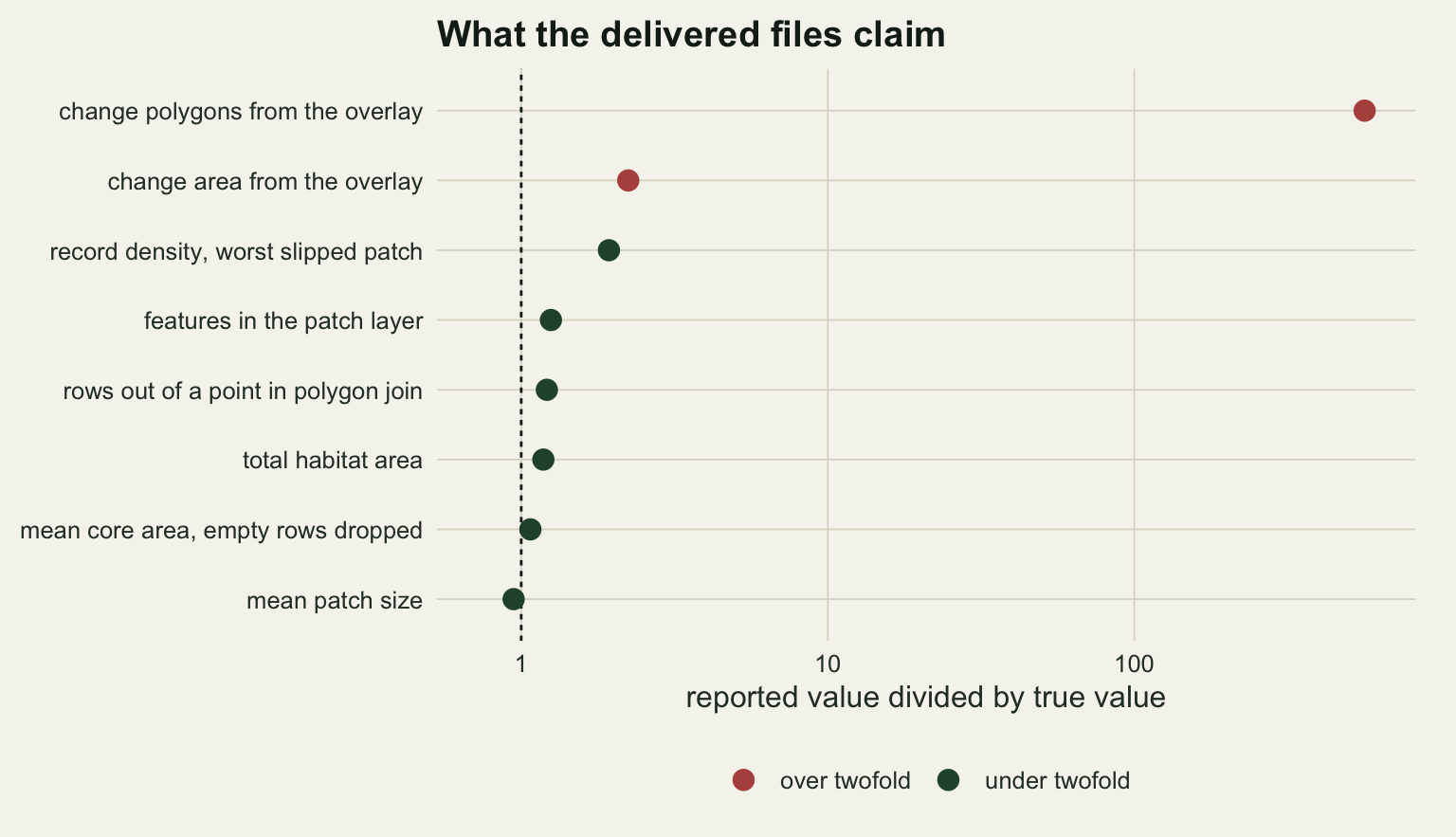
The layer-wide areas, means and row counts are out by a few per cent up to about a quarter. The record density in the worst slipped patch is out by a factor of 1.93 against what the same ground would have reported with a clean outline, the change area from the overlay by more than twofold, and the number of polygons in a change map by more than two orders of magnitude, because a sliver is a whole polygon regardless of how little ground it covers. The two quantities furthest from agreement both come out of an overlay of two layers; the five closest to it are computed over a whole layer at once.
What to report
Give the counts, not the assurance. The number of features, how many were invalid, how much ground was covered twice, how many features had zero or near-zero area, and what was done about each. A methods sentence saying the layer was checked in QGIS is not the same information as a table saying six of seventy five features were invalid and were repaired with st_make_valid.
Do not report a per-patch density screen as a geometry check. The version that separates the slipped patches here scores each one against its own true outline, which a delivered file does not carry, and the version you can compute, against the layer median, is counting noise.
Give the total area both ways when features can overlap: the sum over features and the area of the dissolved union. When those two differ the layer is not a partition of the ground, and every per-hectare quantity computed from the first of them is wrong by their ratio.
Give the row count going into a spatial join and the row count coming out, and if they differ, say which features the extra rows came from. This is the same discipline the attribute-side join asks for and it needs stating separately because no message is printed either way.
For anything built from an overlay of two layers, give the minimum mappable unit and where it came from. The number that matters is not the threshold you chose but the size of the largest artefact the threshold had to remove, because that is the size below which the analysis cannot see.
Give the version of the geometry engine, not only the version of sf. Pebesma (2018) describes sf as a thin R interface over GEOS, GDAL and PROJ: st_make_valid, st_is_valid and the overlay routines are GEOS, and the results here are GEOS 3.13.0. Bivand (2021) traces how much of the R spatial stack’s behaviour is inherited from libraries that version independently of the packages in front of them.
Honest limits
The self-intersections here are one kind: a single vertex swapped with the one opposite it, which produces a large, symmetric crossing and a large cancellation. Real digitising produces small crossings where a boundary has been traced back over itself, and those cancel a few square metres rather than half a patch. The failure mode is identical and the magnitude is not, so the 40.2 per cent figure above demonstrates the mechanism rather than estimating what a real layer loses.
The per-patch diagnosis in the second section is available here and nowhere else. Each slipped patch is scored against the same ground traced correctly, and the correct tracing exists only because the layer was built from it. What a delivered file supports is the comparison against the layer median, and that one is measured above too: a cut low enough to flag all six slipped patches flags 39 of the 54 clean patches with them. The slips in this post are found by the validity scan; the density is what they then move.
The two vegetation maps disagree through a displacement field that is a deterministic function of position, which keeps the second map a clean partition of the block. Two real tracings would also disagree in their vertex counts, would carry their own gaps and overlaps between adjacent units, and would not tile the block at all. That makes the real sliver problem worse than the one measured here, and it adds a failure this post does not touch: gaps, which are slivers with no attributes rather than slivers with two.
Every measurement is planar, in a projected system, on a block small enough that the projection does the right thing. On unprojected data the answers change, sf routes the work through spherical geometry rather than GEOS, and both the validity rules and the overlay behave differently. Which projection to use, and what it costs, is the subject of choosing a projection for area and distance.
The occurrence records are treated as exact points and joined by a strict containment test. Records carry positional error of their own, which moves the failure from the polygon to the point and changes what a join at a boundary means; that is the problem coordinate error and habitat assignment measures, and the two errors compound rather than cancelling.
The scan in check_layer is not free and this post does not measure what it costs. Its first six columns are one pass over the geometry column as delivered; the last two construct geometry, a repair and then a dissolve on top of the repair. On seventy five features none of that is worth thinking about; on a hundred thousand it is, and any figure for it would belong to the machine, the layer and the GEOS build rather than to the method.
References
Pebesma E 2018 The R Journal 10(1):439-446 (10.32614/RJ-2018-009)
Pebesma E, Bivand R 2023 Spatial Data Science: With Applications in R. Chapman and Hall/CRC (ISBN 9780429459016)
MacDougall EB 1975 Landscape Planning 2:23-30 (10.1016/0304-3924(75)90004-0)
Goodchild MF, Hunter GJ 1997 International Journal of Geographical Information Science 11(3):299-306 (10.1080/136588197242419)
Heuvelink GBM, Burrough PA, Stein A 1989 International Journal of Geographical Information Systems 3(4):303-322 (10.1080/02693798908941518)
Shao G, Wu J 2008 Landscape Ecology 23(5):505-511 (10.1007/s10980-008-9215-x)
Bivand R 2021 Journal of Geographical Systems 23(4):515-546 (10.1007/s10109-020-00336-0)