library(ggplot2)
library(patchwork)

te_paper  <- "#f5f4ee"
te_ink    <- "#16241d"
te_body   <- "#2c3a31"
te_forest <- "#275139"
te_rust   <- "#b5534e"
te_gold   <- "#c9b458"
te_line   <- "#dad9ca"

theme_datasheet <- function() {
  theme_minimal(base_size = 12) +
    theme(plot.background  = element_rect(fill = te_paper, colour = NA),
          panel.background = element_rect(fill = te_paper, colour = NA),
          panel.grid.major = element_line(colour = te_line, linewidth = 0.3),
          panel.grid.minor = element_blank(),
          text             = element_text(colour = te_body),
          plot.title       = element_text(colour = te_ink, face = "bold"),
          plot.subtitle    = element_text(colour = te_body),
          axis.text        = element_text(colour = te_body))
}Map accuracy and false fragmentation
R
landscape ecology
remote sensing
simulation
ecology tutorial
At one overall accuracy a land-cover map can give eight times the true patch count or nearly the right one. Which errors do that, and what filters cost, in R.
A regional woodland map arrives with a short metadata sheet: thirty metre pixels, two classes, and an overall accuracy of ninety five per cent from a stratified sample of validation points. The project wants the number of woodland patches, their mean size and the share of woodland in the largest block, because a woodland bird in the study is thought to respond to fragmentation. Ninety five per cent sounds like a map that can carry that analysis, and the accuracy figure is usually the only statement about error the analysis ever quotes.
The accuracy figure counts misclassified pixels. It says nothing about where they are, and fragmentation metrics depend almost entirely on where they are. A wrong pixel in the middle of open farmland is a new woodland patch; a wrong pixel on the edge of a wood moves the edge by one cell and leaves the count alone. This is known: Langford and colleagues 2006 showed with habitat fragmentation examples that map misclassification alone can cause large errors in landscape pattern indices, and Shao and Wu 2008 argued that the accuracy of a pattern analysis has to be assessed in its own right, not read off the accuracy of the map. Nothing below is a new result. It is a demonstration, in base R, of the size of the effect at a fixed accuracy, and of what the usual repair costs.
The site already has the pieces on either side. Patch metrics and fragmentation in R builds the labeller used here, holds habitat amount fixed, and remarks that comparing patch counts between maps made with different classifiers is usually meaningless; it does not measure why. Rasterising a vector layer shows that the cell rule alone can shatter or fuse a woodland network, which is an error made before classification rather than by it. Checking a vector layer before you measure finds that most of the change polygons in an overlay of two map editions are slivers, and that an area threshold removes them at the cost of any real change smaller than the largest sliver; that is the vector version of the trade-off measured at the end of this post. Coordinate error and habitat assignment moves the records rather than the map. Here the map itself is wrong, by the same overall amount, in three different ways.
A true landscape and three ways to misclassify it
The true landscape is a continuous suitability score on a 150 by 150 grid, uniform noise smoothed by ten passes of a local average and standardised, thresholded at its 60th percentile so that exactly forty per cent of cells are woodland. The score stands in for whatever a classifier computes before it assigns a class: a spectral index, a posterior probability, a distance in feature space. Patches are four-connected and labelled by label propagation, as in the patch metrics post, with a pointer-jumping step added so that long, winding patches need far fewer sweeps to converge.
The three error models are all calibrated to the same expected overall accuracy.
The first flips each pixel independently with probability one minus the accuracy. This is the textbook error model and the one an accuracy figure implicitly describes: every pixel equally likely to be wrong.
The second adds independent Gaussian noise to the score of every pixel before thresholding. A pixel whose true score sits far from the threshold is almost never flipped; a pixel on the edge of a wood is flipped often. The errors are still pixel by pixel, but they are concentrated along class boundaries, which is what a per-pixel classifier does with mixed and transitional pixels.
The third adds the same amount of noise, but correlated between neighbouring cells: Gaussian noise smoothed by four passes and rescaled to the same marginal standard deviation. Its correlation range, measured just below, is a few cells, shorter than the woodland pattern itself, so a short run of boundary moves together where the second model moves single cells. It is not a model of a slowly varying illumination or phenology gradient, which would shift boundaries over distances far larger than a patch.
For both score-noise models the expected error rate has a closed form, the mean over cells of the normal probability that noise carries the score across the threshold, so the noise standard deviation that gives a target accuracy is found by one call to uniroot without any simulation.
n_side <- 150; amount <- 0.4          # grid side, true woodland share
field_passes <- 10; noise_passes <- 4 # smoothing of truth and of correlated noise
acc_set <- c(0.98, 0.95, 0.90)        # target overall accuracies
n_maps <- 20                          # true landscapes per cell, fixed in advance
mmu_cells <- 5                        # minimum mapping unit of the sieve
mmu_grid <- 1:12
model_lev <- c("independent pixels", "pixel score noise", "correlated score noise")

smooth_pass <- function(z) {
  n <- nrow(z)
  pad <- rbind(z[1, ], z, z[n, ]); pad <- cbind(pad[, 1], pad, pad[, n])
  (pad[1:n, 2:(n + 1)] + pad[3:(n + 2), 2:(n + 1)] + pad[2:(n + 1), 1:n] +
     pad[2:(n + 1), 3:(n + 2)] + 4 * pad[2:(n + 1), 2:(n + 1)]) / 8
}
smooth_field <- function(n, k, gen) {
  z <- matrix(gen(n * n), n)
  for (i in seq_len(k)) z <- smooth_pass(z)
  (z - mean(z)) / sd(z)
}
label_patches <- function(hab) {
  n <- nrow(hab); m <- ncol(hab)
  lab <- matrix(0L, n, m); idx <- which(hab); lab[idx] <- idx
  repeat {
    old <- lab
    best <- pmax(lab, rbind(0L, lab[-n, ]), rbind(lab[-1, ], 0L),
                 cbind(0L, lab[, -m]), cbind(lab[, -1], 0L))
    lab[idx] <- best[idx]
    for (k in 1:3) lab[idx] <- lab[lab[idx]]   # pointer jumping
    if (identical(lab, old)) break
  }
  lab
}
patch_sizes <- function(lab) tabulate(lab[lab > 0], nbins = length(lab))
metrics_of <- function(hab, lab = label_patches(hab)) {
  n <- nrow(hab); s <- patch_sizes(lab); s <- s[s > 0]
  c(patches = length(s), mean_size = mean(s), lpi = max(s) / sum(hab),
    edge = (sum(hab[-n, ] != hab[-1, ]) + sum(hab[, -n] != hab[, -1])) / n^2,
    singles = sum(s == 1))
}
exp_err <- function(z, thr, s) mean(pnorm(-abs(z - thr) / s))
make_truth <- function() {
  z <- smooth_field(n_side, field_passes, runif)
  thr <- quantile(z, 1 - amount)
  list(z = z, thr = thr, truth = z >= thr)
}
misclassify <- function(tl, acc) {
  e <- 1 - acc
  s <- uniroot(function(s) exp_err(tl$z, tl$thr, s) - e, c(1e-4, 5), tol = 1e-8)$root
  list(xor(tl$truth, matrix(runif(n_side^2) < e, n_side)),
       (tl$z + rnorm(n_side^2, 0, s)) >= tl$thr,
       (tl$z + s * smooth_field(n_side, noise_passes, rnorm)) >= tl$thr)
}
lag_cor <- function(z, lag) cor(as.vector(z[, 1:(n_side - lag)]), as.vector(z[, (1 + lag):n_side]))
set.seed(31604)
noise_cor <- vapply(1:6, lag_cor, 0, z = smooth_field(n_side, noise_passes, rnorm))
field_z <- smooth_field(n_side, field_passes, runif)
field_cor <- vapply(1:6, lag_cor, 0, z = field_z)
field_hab <- field_z >= quantile(field_z, 1 - amount)
pad_hab <- rbind(field_hab[1, ], field_hab, field_hab[n_side, ])
pad_hab <- cbind(pad_hab[, 1], pad_hab, pad_hab[, n_side])
mid <- 2:(n_side + 1)
on_edge <- (pad_hab[mid - 1, mid] != field_hab) | (pad_hab[mid + 1, mid] != field_hab) |
(pad_hab[mid, mid - 1] != field_hab) | (pad_hab[mid, mid + 1] != field_hab)
edge_share <- mean(on_edge)
round(rbind(noise = noise_cor, true_score = field_cor), 2) [,1] [,2] [,3] [,4] [,5] [,6]
noise 0.77 0.37 0.12 0.02 0.0 0.00
true_score 0.91 0.67 0.41 0.21 0.1 0.04Along a row of cells the correlated noise has a correlation of 0.77 between neighbours, 0.37 at two cells, 0.12 at three and 0.02 at four. The true score field it is added to keeps 0.41 at three cells and falls to 0.10 at five. The error is correlated over two or three cells, a shorter range than the pattern it distorts.
One landscape, misclassified once by each model at ninety five per cent, is enough to see the difference.
set.seed(31605)
ex_tl <- make_truth()
ex_obs <- misclassify(ex_tl, 0.95)
ex_maps <- c(list(ex_tl$truth), ex_obs)
ex_names <- c("error-free", model_lev)
ex_acc <- vapply(ex_obs, function(o) mean(o == ex_tl$truth), 0)
ex_np <- vapply(ex_maps, function(h) metrics_of(h)[["patches"]], 0)
The error-free map has 107 woodland patches. At realised accuracies of 0.952, 0.952 and 0.949, the three misclassified versions have 522, 171 and 121 patches. Three maps that would pass the same accuracy assessment disagree about the patch count by a factor of 4.3.
cell_df <- do.call(rbind, lapply(seq_along(ex_maps), function(i) {
  h <- ex_maps[[i]]; tr <- ex_tl$truth
  state <- ifelse(h & tr, "woodland", ifelse(h & !tr, "false woodland",
                  ifelse(!h & tr, "missed woodland", "open")))
  data.frame(x = rep(seq_len(n_side), each = n_side), y = rep(seq_len(n_side), n_side),
             state = as.vector(state),
             panel = sprintf("%s: %.0f patches", ex_names[i], ex_np[i]))
}))
cell_df$panel <- factor(cell_df$panel, levels = unique(cell_df$panel))
cell_df <- cell_df[cell_df$state != "open", ]
ggplot(cell_df, aes(x, y, fill = state)) +
  geom_raster() +
  facet_wrap(~panel, ncol = 2) +
  coord_equal(expand = FALSE) +
  scale_fill_manual(values = c(woodland = te_forest, `false woodland` = te_rust,
                               `missed woodland` = te_gold), name = NULL) +
  labs(x = NULL, y = NULL, title = "Four maps, three of them 95 per cent correct") +
  theme_datasheet() +
  theme(axis.text = element_blank(), panel.grid = element_blank(),
        strip.text = element_text(colour = te_ink, hjust = 0),
        legend.position = "bottom")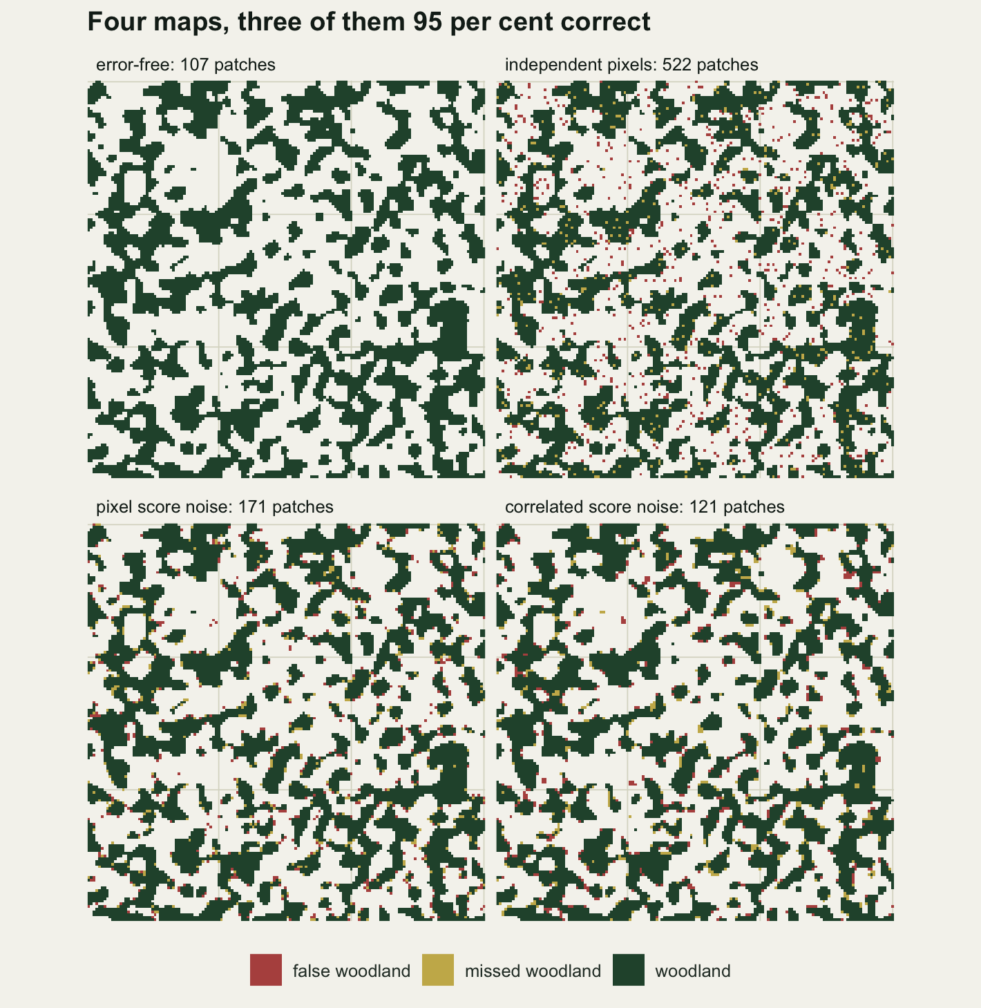
The patch count follows the kind of error
One map is an anecdote. The simulation below draws 20 true landscapes, a number fixed before any result was seen, and misclassifies each of them by each model at each of the three accuracies. Every metric is reported as a ratio to the same landscape’s error-free value, so the variation between landscapes cancels. The repair columns used later in the post are computed in the same pass, so that every number comes from the same maps.
majority3 <- function(hab) {
  n <- nrow(hab); p <- rbind(hab[1, ], hab, hab[n, ]); p <- cbind(p[, 1], p, p[, n])
  s <- 0
  for (di in 0:2) for (dj in 0:2) s <- s + p[1:n + di, 1:n + dj]
  s >= 5
}
sieve <- function(hab, mmu, lab = label_patches(hab)) {
  s <- patch_sizes(lab)
  out <- hab; out[hab & s[pmax(lab, 1L)] < mmu] <- FALSE
  mlab <- label_patches(!out); ms <- patch_sizes(mlab)
  out[!out & ms[pmax(mlab, 1L)] < mmu] <- TRUE
  out
}
exp_singles <- function(truth, e) {
  n <- nrow(truth); p_h <- ifelse(truth, 1 - e, e)
  pad <- matrix(1, n + 2, n + 2); pad[2:(n + 1), 2:(n + 1)] <- 1 - p_h
  sum(p_h * pad[1:n, 2:(n + 1)] * pad[3:(n + 2), 2:(n + 1)] *
        pad[2:(n + 1), 1:n] * pad[2:(n + 1), 3:(n + 2)])
}
audit <- function(truth, tlab, rep_map) {
  rlab <- label_patches(rep_map)
  kept <- unique(tlab[truth & rep_map]); real <- unique(rlab[truth & rep_map])
  c(metrics_of(rep_map, rlab),
    lost = length(setdiff(unique(tlab[tlab > 0]), kept)),
    false = length(setdiff(unique(rlab[rlab > 0]), real)),
    acc = mean(rep_map == truth))
}
mmu_curve <- function(truth, tlab, o, olab, label) {
  s <- patch_sizes(olab); s_pos <- s[s > 0]
  idx <- which(truth & o)
  best <- tapply(s[olab[idx]], factor(tlab[idx], levels = unique(tlab[tlab > 0])), max)
  best[is.na(best)] <- 0
  data.frame(mmu = mmu_grid, map = label,
             patches = vapply(mmu_grid, function(k) sum(s_pos >= k), 0),
             lost = vapply(mmu_grid, function(k) mean(best < k), 0))
}
one_map <- function(seed) {
  set.seed(seed)
  tl <- make_truth(); truth <- tl$truth
  tlab <- label_patches(truth); tm <- metrics_of(truth, tlab)
  rows <- list(data.frame(map = seed, target = 1, model = "error-free", acc = 1, t(tm),
                          maj = t(audit(truth, tlab, majority3(truth))),
                          sv = t(audit(truth, tlab, sieve(truth, mmu_cells, tlab))),
                          exp_singles = NA))
  curves <- list(mmu_curve(truth, tlab, truth, tlab, "error-free"))
  for (a in acc_set) {
    obs <- misclassify(tl, a)
    for (k in 1:3) {
      o <- obs[[k]]; olab <- label_patches(o)
      rows[[length(rows) + 1]] <- data.frame(map = seed, target = a, model = model_lev[k],
        acc = mean(o == truth), t(metrics_of(o, olab)),
        maj = t(audit(truth, tlab, majority3(o))),
        sv = t(audit(truth, tlab, sieve(o, mmu_cells, olab))),
        exp_singles = if (k == 1) exp_singles(truth, 1 - a) else NA)
      if (a == 0.95) curves[[length(curves) + 1]] <- mmu_curve(truth, tlab, o, olab, model_lev[k])
    }
  }
  list(rows = do.call(rbind, rows), curves = do.call(rbind, curves))
}
runs <- lapply(4100 + seq_len(n_maps), one_map)
sim <- do.call(rbind, lapply(runs, `[[`, "rows"))
curves <- do.call(rbind, lapply(runs, `[[`, "curves"))

base <- sim[sim$model == "error-free", ]
err <- sim[sim$model != "error-free", ]
m_row <- match(err$map, base$map)
for (v in c("patches", "mean_size", "lpi", "edge")) err[[paste0("r_", v)]] <- err[[v]] / base[[v]][m_row]
cell_mean <- function(v, mod, a) mean(err[[v]][err$model == mod & err$target == a])
cell_se <- function(v, mod, a) { x <- err[[v]][err$model == mod & err$target == a]; sd(x) / sqrt(length(x)) }
cell_sd <- function(v, mod, a) sd(err[[v]][err$model == mod & err$target == a])
true_np <- mean(base$patches); true_np_rng <- range(base$patches)
acc_dev <- max(abs(err$acc - err$target))
The error-free landscapes have 110.7 patches on average, between 94 and 124. Realised accuracy never strays more than 0.0056 from its target in any of the misclassified maps, so the three models really are being compared at the same accuracy.
At ninety eight per cent accuracy, independent pixel errors multiply the patch count by 2.66, pixel score noise by 1.06 and correlated score noise by 1.01. At ninety five per cent the three factors are 4.94, 1.52 and 1.03; at ninety per cent they are 8.10, 3.36 and 1.13. The largest standard error across landscapes in any of these nine cells is 0.146, so the ordering is not noise. A map that is ninety per cent correct with correlated errors has a more trustworthy patch count than a map that is ninety eight per cent correct with independent ones.
ind <- err[err$model == model_lev[1], ]
single_tab <- aggregate(cbind(singles, exp_singles) ~ target, ind, mean)
single_gap <- max(abs(single_tab$singles - single_tab$exp_singles) / single_tab$exp_singles)
excess_tab <- aggregate(patches ~ target, ind, mean)
excess_tab$excess <- excess_tab$patches - true_np
excess_tab$single_share <- (single_tab$singles - mean(base$singles)) / excess_tab$excess
single_tab
target singles exp_singles
1 0.90 655.70 654.3662
2 0.95 402.85 395.8730
3 0.98 182.55 180.0624The independent-pixel arm is close to arithmetic, and it should be checked as arithmetic rather than admired as a finding. Under independent flips a cell is a one-cell patch when it is observed as woodland and all four of its neighbours are observed as open ground, and each of those events has a known probability, so the expected number of one-cell patches is a sum over cells of a product of five probabilities. The closed form predicts 180, 396 and 654 single-cell patches at the three accuracies from high to low; the simulation gives 183, 403 and 656, a largest relative gap of 0.018. Single cells account for 96, 91 and 83 per cent of the extra patches; the rest are pairs and small clusters of wrong cells, and fragments cut off true patches. The score-noise arms have no such shortcut, because whether a wrong cell is isolated depends on how the true score varies around it.
count_tab <- aggregate(r_patches ~ model + target, err, function(x) c(m = mean(x), se = sd(x) / sqrt(length(x))))
count_tab <- data.frame(model = factor(count_tab$model, levels = model_lev), target = count_tab$target,
                        m = count_tab$r_patches[, "m"], se = count_tab$r_patches[, "se"])
ggplot(count_tab, aes(target, m, colour = model)) +
  geom_hline(yintercept = 1, colour = te_body, linetype = "dashed", linewidth = 0.5) +
  geom_line(linewidth = 0.9) +
  geom_errorbar(aes(ymin = m - 2 * se, ymax = m + 2 * se), width = 0.004, linewidth = 0.5) +
  geom_point(size = 2.4) +
  scale_x_reverse(breaks = acc_set, labels = c("0.98", "0.95", "0.90")) +
  scale_y_log10(breaks = c(1, 1.5, 2, 3, 5, 8)) +
  scale_colour_manual(values = c(te_rust, te_gold, te_forest), name = NULL) +
  labs(x = "overall accuracy", y = "patch count / true patch count (log scale)",
       title = "Same accuracy, different landscapes",
       subtitle = "dashed line: the error-free patch count") +
  theme_datasheet() + theme(legend.position = "bottom")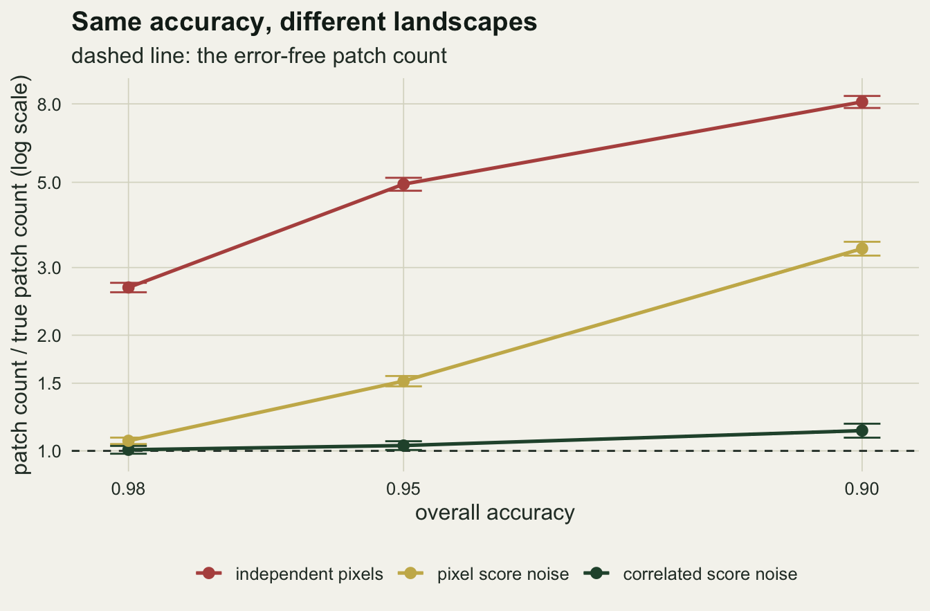
Sparing the count does not spare the largest patch
Patch count is the metric most exposed to isolated errors. Edge density is exposed to them too, and the largest-patch index, the share of all woodland in the biggest patch, reacts to something else: whether a thin neck of woodland is cut, or a narrow gap is closed.
shape_val <- function(v) sapply(acc_set, function(a) vapply(model_lev, function(m) cell_mean(v, m, a), 0))
edge_r <- shape_val("r_edge"); size_r <- shape_val("r_mean_size"); lpi_r <- shape_val("r_lpi")
lpi_sd <- sapply(acc_set, function(a) vapply(model_lev, function(m) cell_sd("r_lpi", m, a), 0))
off_band <- function(mod, a) {
  x <- err$r_lpi[err$model == mod & err$target == a]
  mean(x < 0.8 | x > 1.25)
}
band_90 <- vapply(model_lev, off_band, 0, a = 0.90)
band_95 <- vapply(model_lev, off_band, 0, a = 0.95)
band_98 <- vapply(model_lev, off_band, 0, a = 0.98)
band_se <- sqrt(0.25 / n_maps)
lpi_true_rng <- range(base$lpi)
At ninety per cent, independent errors multiply edge density by 1.97 and cut mean patch size to 0.13 of its true value; pixel score noise gives 1.42 and 0.30; correlated score noise gives 1.07 and 0.90. Mean patch size is the reciprocal of patch density at fixed habitat amount, so it carries the count result over almost unchanged.
The largest-patch index behaves differently. Averaged over landscapes, its ratio to the truth at ninety per cent is 0.73 for independent errors, 0.78 for pixel score noise and 1.03 for correlated score noise. The average hides the spread. Across the 20 landscapes the standard deviation of that ratio is 0.18, 0.32 and 0.51, so correlated error leaves the average alone and scatters the individual maps widely.
Call a largest-patch index wrong when the misclassified map puts it more than a fifth below or a quarter above the truth. At ninety per cent accuracy the share of landscapes with a wrong index is 0.65 for independent errors, 0.55 for pixel score noise and 0.55 for correlated score noise: at that accuracy every error model gets it wrong in about half the maps or more. At ninety five per cent the shares are 0.15, 0.20 and 0.55, and at ninety eight per cent 0.10, 0.20 and 0.25. With 20 landscapes each share has a Monte Carlo standard error of up to 0.11, which is too coarse to rank the models. The comparison is therefore repeated on 120 further landscapes at the two higher accuracies, a number set by the time budget before the run. Each landscape is misclassified by all three models, so the comparison is paired: the Monte Carlo error of a difference comes from the per-landscape differences, and the exact McNemar test uses only the landscapes on which two models disagree.
n_lpi <- 120                          # extra landscapes for the paired check, fixed in advance
lpi_check <- function(seed) {
  set.seed(seed)
  tl <- make_truth(); t_lpi <- metrics_of(tl$truth)[["lpi"]]
  rows <- NULL
  for (a in c(0.98, 0.95)) {
    obs <- misclassify(tl, a)
    for (k in 1:3) {
      o <- obs[[k]]; lab1 <- label_patches(o); s1 <- patch_sizes(lab1)
      small_err <- small_ok <- NA
      if (a == 0.95) {                  # size of the mapped patch, of either class, holding each cell
        lab0 <- label_patches(!o); s0 <- patch_sizes(lab0)
        home <- ifelse(o, s1[pmax(lab1, 1L)], s0[pmax(lab0, 1L)])
        wrong <- o != tl$truth
        small_err <- mean(home[wrong] < mmu_cells); small_ok <- mean(home[!wrong] < mmu_cells)
      }
      rows <- rbind(rows, data.frame(map = seed, target = a, model = model_lev[k],
                                     r_lpi = max(s1) / sum(o) / t_lpi, small_err, small_ok))
    }
  }
  rows
}
chk <- do.call(rbind, lapply(7000 + seq_len(n_lpi), lpi_check))
chk$off <- chk$r_lpi < 0.8 | chk$r_lpi > 1.25
pair_test <- function(a, m1, m2) {
  x <- chk$off[chk$target == a & chk$model == m1]; y <- chk$off[chk$target == a & chk$model == m2]
  d <- x - y; only1 <- sum(x & !y); only2 <- sum(y & !x)
  c(share1 = mean(x), share2 = mean(y), diff = mean(d), se = sd(d) / sqrt(length(d)),
    only1 = only1, only2 = only2, p = binom.test(only1, only1 + only2)$p.value)
}
pairs_tab <- rbind(
  cor_pix_95 = pair_test(0.95, model_lev[3], model_lev[2]),
  cor_ind_95 = pair_test(0.95, model_lev[3], model_lev[1]),
  pix_ind_95 = pair_test(0.95, model_lev[2], model_lev[1]),
  cor_pix_98 = pair_test(0.98, model_lev[3], model_lev[2]),
  cor_ind_98 = pair_test(0.98, model_lev[3], model_lev[1]),
  pix_ind_98 = pair_test(0.98, model_lev[2], model_lev[1]))
pt <- function(r, col) pairs_tab[r, col]
share_chk <- function(m, a) mean(chk$off[chk$model == m & chk$target == a])
small_tab <- aggregate(cbind(small_err, small_ok) ~ model, chk[chk$target == 0.95, ], mean)
small_tab <- small_tab[match(model_lev, small_tab$model), ]
round(pairs_tab, 3)
share1 share2 diff se only1 only2 p
cor_pix_95 0.383 0.308 0.075 0.059 30 21 0.262
cor_ind_95 0.383 0.183 0.200 0.060 40 16 0.002
pix_ind_95 0.308 0.183 0.125 0.054 29 14 0.032
cor_pix_98 0.225 0.125 0.100 0.042 19 7 0.029
cor_ind_98 0.225 0.058 0.167 0.045 26 6 0.001
pix_ind_98 0.125 0.058 0.067 0.039 15 7 0.134On these landscapes the largest-patch index is wrong at ninety five per cent in 0.18 of maps for independent errors, 0.31 for pixel score noise and 0.38 for correlated score noise, and at ninety eight per cent in 0.06, 0.12 and 0.23. Correlated score noise gets the index wrong more often than independent errors at both accuracies: the paired difference is 0.200 (standard error 0.060, McNemar p = 0.002) at ninety five per cent and 0.167 (0.045, p = 0.001) at ninety eight. Pixel score noise sits between the two: 0.125 (0.054, p = 0.032) and 0.067 (0.039, p = 0.134) above independent errors. Between the two score-noise models the difference is 0.075 (0.059, p = 0.262) at ninety five per cent and 0.100 (0.042, p = 0.029) at ninety eight. So the errors that spare the patch count leave the largest-patch index wrong at least as often as independent errors do, and the correlated kind more often; whether correlated noise is worse than pixel score noise is not settled here: one of those two differences is more than two standard errors from zero and the other is not, and the ordering in the twenty landscapes of the main simulation should not be read as more than that. In those twenty landscapes the true largest-patch index itself runs from 0.084 to 0.392: at forty per cent woodland the largest patches are joined to their neighbours by narrow necks, and a boundary that moves by a few cells over a stretch of map can open or close one of them.
edge_tab <- aggregate(r_edge ~ model + target, err, mean)
edge_tab$model <- factor(edge_tab$model, levels = model_lev)
p_edge <- ggplot(edge_tab, aes(target, r_edge, colour = model)) +
  geom_hline(yintercept = 1, colour = te_body, linetype = "dashed", linewidth = 0.5) +
  geom_line(linewidth = 0.9, show.legend = FALSE) + geom_point(size = 2.2) +
  scale_x_reverse(breaks = acc_set, labels = c("0.98", "0.95", "0.90")) +
  scale_colour_manual(values = c(te_rust, te_gold, te_forest), name = NULL) +
  guides(colour = guide_legend(override.aes = list(size = 3, alpha = 1))) +
  labs(x = "overall accuracy", y = "edge density / truth", title = "Edge density") +
  theme_datasheet() + theme(legend.position = "none")
lpi_pts <- err
lpi_pts$model <- factor(lpi_pts$model, levels = model_lev)
lpi_pts$acc_lab <- factor(sprintf("%.2f", lpi_pts$target), levels = c("0.98", "0.95", "0.90"))
p_lpi <- ggplot(lpi_pts, aes(acc_lab, r_lpi, colour = model)) +
  annotate("rect", xmin = -Inf, xmax = Inf, ymin = 0.8, ymax = 1.25, fill = te_line, alpha = 0.6) +
  geom_hline(yintercept = 1, colour = te_body, linetype = "dashed", linewidth = 0.5) +
  geom_point(position = position_jitterdodge(jitter.width = 0.12, dodge.width = 0.75, seed = 7),
             size = 1.5, alpha = 0.8, show.legend = FALSE) +
  scale_y_log10(breaks = c(0.3, 0.5, 0.8, 1, 1.25, 2)) +
  scale_colour_manual(values = c(te_rust, te_gold, te_forest), name = NULL) +
  labs(x = "overall accuracy", y = "largest-patch index / truth (log scale)",
       title = "Largest-patch index") +
  theme_datasheet() + theme(legend.position = "bottom")
(p_edge + p_lpi + plot_layout(guides = "collect") +
  plot_annotation(theme = theme_datasheet() + theme(legend.position = "bottom"))) &
  theme(legend.position = "bottom")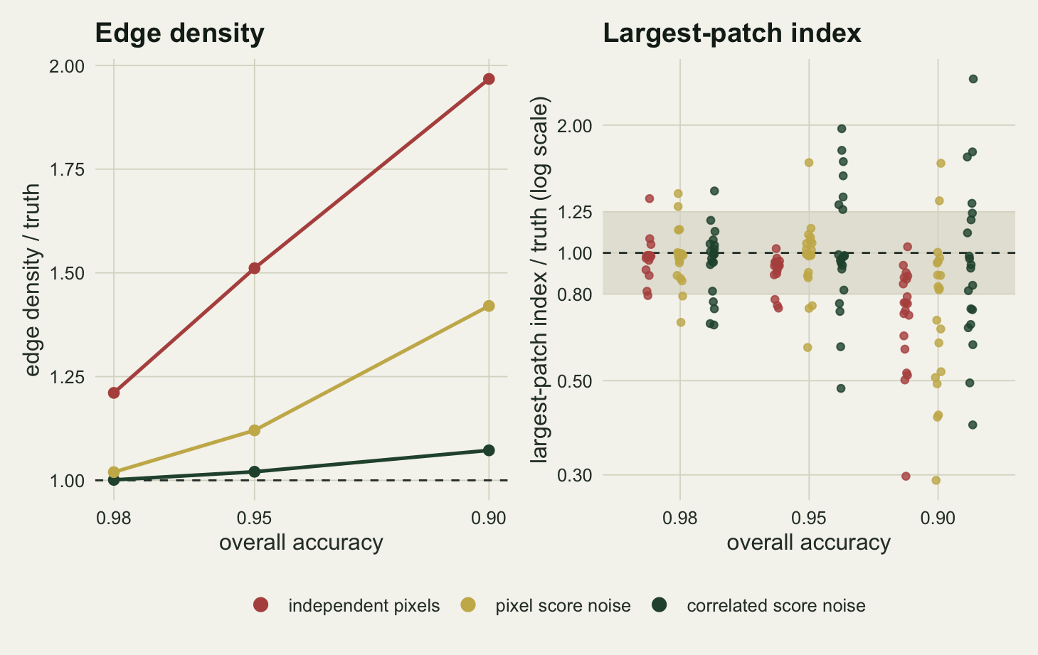
A majority filter trades false patches for real ones
The standard response to a speckled map is to smooth it. A three by three majority filter replaces each cell with the class held by at least five of the nine cells in its window; a sieve, the minimum mapping unit, removes every patch of either class smaller than a set number of cells and gives it to the surrounding class. Both bring the count to somewhat below the truth, whatever it was before. The question is what that count is made of.
rep_val <- function(v, mod, a) {
  if (mod == "error-free") return(mean(base[[v]]))
  mean(err[[v]][err$model == mod & err$target == a])
}
maj_free <- rep_val("maj.patches", "error-free"); sv_free <- rep_val("sv.patches", "error-free")
maj_free_lost <- rep_val("maj.lost", "error-free"); sv_free_lost <- rep_val("sv.lost", "error-free")
maj_free_acc <- rep_val("maj.acc", "error-free"); sv_free_acc <- rep_val("sv.acc", "error-free")
maj_cells <- expand.grid(model = model_lev, target = acc_set, stringsAsFactors = FALSE)
maj_cells$patches <- mapply(function(m, a) rep_val("maj.patches", m, a), maj_cells$model, maj_cells$target)
maj_cells$lost <- mapply(function(m, a) rep_val("maj.lost", m, a), maj_cells$model, maj_cells$target)
maj_cells$false <- mapply(function(m, a) rep_val("maj.false", m, a), maj_cells$model, maj_cells$target)
maj_cells$acc_after <- mapply(function(m, a) rep_val("maj.acc", m, a), maj_cells$model, maj_cells$target)
maj_cells$sv_patches <- mapply(function(m, a) rep_val("sv.patches", m, a), maj_cells$model, maj_cells$target)
maj_cells$sv_lost <- mapply(function(m, a) rep_val("sv.lost", m, a), maj_cells$model, maj_cells$target)
maj_cells$sv_false <- mapply(function(m, a) rep_val("sv.false", m, a), maj_cells$model, maj_cells$target)
maj_cells$sv_acc <- mapply(function(m, a) rep_val("sv.acc", m, a), maj_cells$model, maj_cells$target)
mc <- function(col, m, a) maj_cells[[col]][maj_cells$model == m & maj_cells$target == a]
lost_rng <- range(maj_cells$lost); sv_lost_rng <- range(maj_cells$sv_lost)
print(format(maj_cells, digits = 3), row.names = FALSE)
model target patches lost false acc_after sv_patches sv_lost
independent pixels 0.98 90.8 18.9 0.10 0.964 90.0 20.9
pixel score noise 0.98 88.8 19.5 0.10 0.962 89.1 20.2
correlated score noise 0.98 89.2 19.5 0.00 0.960 89.2 20.3
independent pixels 0.95 92.0 18.2 0.60 0.955 92.5 19.7
pixel score noise 0.95 90.8 18.2 0.20 0.949 92.5 19.7
correlated score noise 0.95 90.0 17.1 0.70 0.940 89.3 16.8
independent pixels 0.90 99.2 17.4 5.65 0.938 100.3 19.4
pixel score noise 0.90 98.2 16.9 2.55 0.931 102.0 19.2
correlated score noise 0.90 93.2 15.5 3.70 0.901 93.0 15.2
sv_false sv_acc
0.00 0.989
0.00 0.978
0.00 0.978
0.00 0.977
0.05 0.951
0.15 0.949
1.10 0.953
0.80 0.914
2.15 0.901# which true patches does the filter delete from an error-free map
set.seed(4101)
tl_chk <- make_truth(); tlab_chk <- label_patches(tl_chk$truth)
ts <- patch_sizes(tlab_chk)
ids_chk <- unique(tlab_chk[tlab_chk > 0])
kept_chk <- unique(tlab_chk[tl_chk$truth & majority3(tl_chk$truth)])
lost_sizes <- ts[setdiff(ids_chk, kept_chk)]; kept_sizes <- ts[kept_chk]Applied to the error-free maps, where there is nothing to repair, the majority filter returns 90.2 patches against a true 110.7. It has deleted 19.2 real patches per map, 17 per cent of them, and lowered the overall accuracy of a perfect map to 0.970 by rounding off corners and cutting narrow necks. The filter does not work by size alone: in the first landscape the largest true patch it removed had 5 cells, while the smallest that still had a woodland cell afterwards had 3. A patch of three cells can keep a cell only when cells of other patches fall inside the same three by three window, so what the filter deletes depends on the neighbours of a patch as well as its size. The sieve with a minimum mapping unit of 5 cells returns 89.8 patches, deletes 20.9 real patches, which by construction are exactly the true patches below the unit, and leaves accuracy at 0.997.
On the misclassified maps the filtered counts lie between 88.8 and 99.2 for every model and accuracy, and the sieved counts between 89.1 and 102.0. That agreement is the problem. The filter deletes between 15.5 and 19.5 true patches per map whatever the input, and the sieve between 15.2 and 20.9. On the worst map, ninety per cent correct with independent errors, the filtered count of 99.2 is the truth, minus 17.4 real patches, plus 5.7 patches that contain no true woodland at all, plus the balance of merges and splits. A count of that size built from two errors that partly offset each other is not a repaired count.
The filter does not improve accuracy either, except where there was a great deal to improve. On the independent-error maps it moves accuracy from 0.98 to 0.964 and from 0.90 to 0.938. The sieve does better on both, 0.989 and 0.953, because it leaves the boundaries of large patches alone.
curve_tab <- aggregate(cbind(patches, lost) ~ mmu + map, curves, mean)
curve_tab$map <- factor(curve_tab$map, levels = c("error-free", model_lev))
cv <- function(col, m, k) curve_tab[[col]][curve_tab$map == m & curve_tab$mmu == k]
first_ok <- function(m) min(curve_tab$mmu[curve_tab$map == m & abs(curve_tab$patches / cv("patches", "error-free", 1) - 1) <= 0.1])
mmu_need <- vapply(model_lev, first_ok, 0)
sieve_gap <- max(abs(vapply(c("error-free", model_lev), function(m) cv("patches", m, mmu_cells), 0) -
  c(sv_free, vapply(model_lev, function(m) mc("sv_patches", m, 0.95), 0))))
The minimum mapping unit is a dial, so the trade-off can be drawn as a curve. The sweep below removes woodland patches below each unit from one to twelve cells on the ninety five per cent maps, without the matching fill of small open-ground holes; at the unit of 5 cells this shortcut lands within 2.6 patches of the full two-class sieve. The smallest unit that brings the count within ten per cent of the true count is 3 cells for independent errors, 2 for pixel score noise and 1 for correlated score noise. For correlated error a unit of one cell is no sieve at all. At those units the share of true patches that no longer exist anywhere on the map is 0.10, 0.06 and 0.04; part of that loss is done by the misclassification itself, before any sieve, since a small true patch can be erased by the error. The error-free curve shows the same deletion with no error to remove: 0.19 of true patches gone at 5 cells and 0.40 at 12.
curve_tab$r_patches <- curve_tab$patches / cv("patches", "error-free", 1)
pal4 <- c(`error-free` = te_ink, `independent pixels` = te_rust,
          `pixel score noise` = te_gold, `correlated score noise` = te_forest)
p_cnt <- ggplot(curve_tab, aes(mmu, r_patches, colour = map)) +
  geom_hline(yintercept = 1, colour = te_body, linetype = "dashed", linewidth = 0.5) +
  geom_line(linewidth = 0.9) + geom_point(size = 1.6) +
  scale_y_log10(breaks = c(0.6, 0.8, 1, 1.5, 2, 3, 5)) +
  scale_x_continuous(breaks = c(1, 3, 5, 7, 9, 11)) +
  scale_colour_manual(values = pal4, name = NULL) +
  labs(x = "minimum mapping unit (cells)", y = "patch count / truth (log scale)",
       title = "The count comes back") +
  theme_datasheet()
p_lost <- ggplot(curve_tab, aes(mmu, lost, colour = map)) +
  geom_line(linewidth = 0.9) + geom_point(size = 1.6) +
  scale_x_continuous(breaks = c(1, 3, 5, 7, 9, 11)) +
  scale_colour_manual(values = pal4, name = NULL) +
  labs(x = "minimum mapping unit (cells)", y = "share of true patches deleted",
       title = "Real patches go with it") +
  theme_datasheet()
p_cnt <- p_cnt + guides(colour = guide_legend(nrow = 2))
p_lost <- p_lost + guides(colour = guide_legend(nrow = 2))
(p_cnt + p_lost + plot_layout(guides = "collect") +
  plot_annotation(theme = theme_datasheet() + theme(legend.position = "bottom"))) &
  theme(legend.position = "bottom")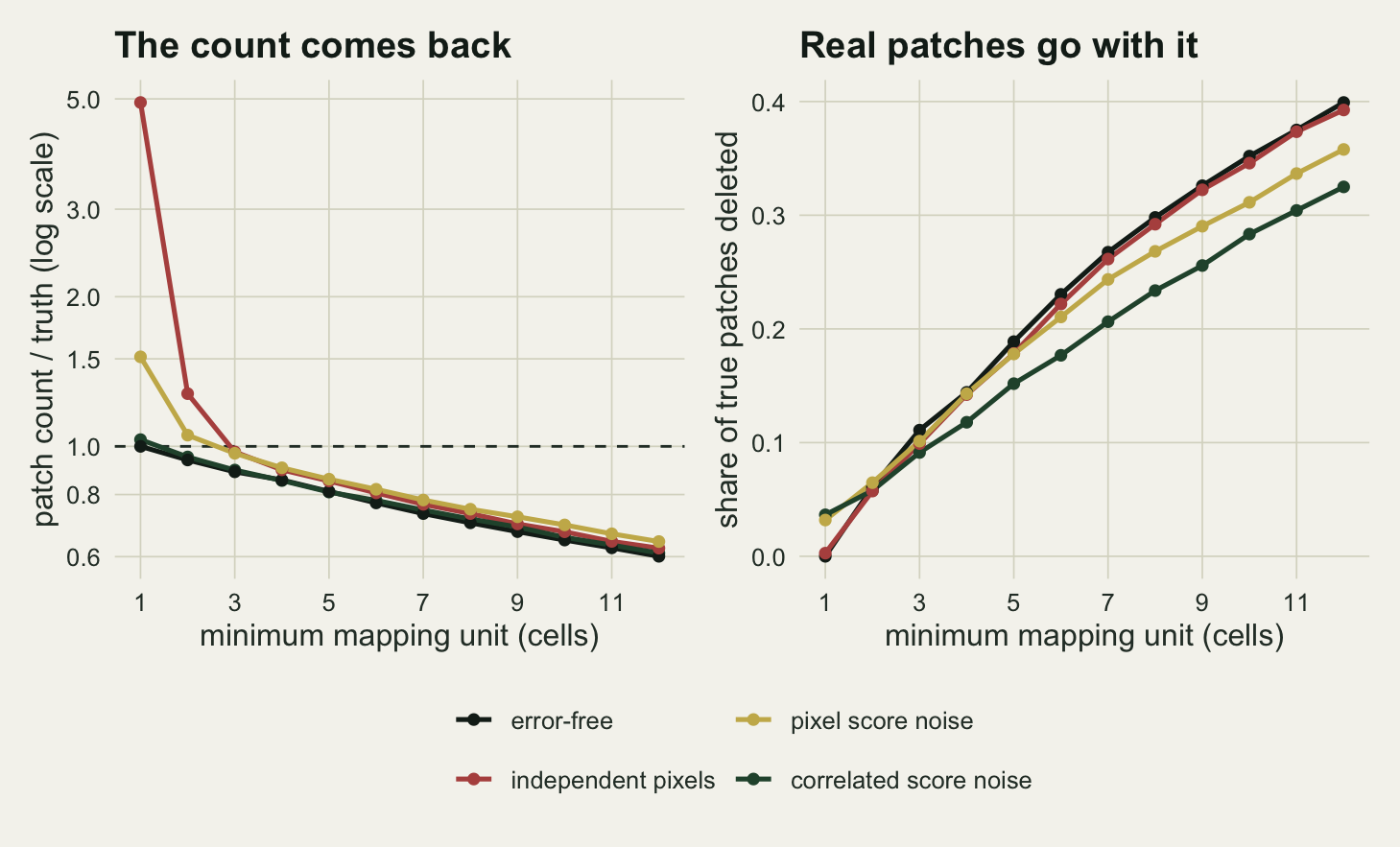
What to report
Report the overall accuracy, and do not let it stand in for the accuracy of the fragmentation metrics. The measurements here say that the same accuracy is compatible with a patch count close to the truth and with one several times too high, depending on where the errors fall. If the classifier’s validation points exist, the cheapest extra evidence is where the wrong ones fall. Distance to a mapped boundary does not separate the error models, because an isolated wrong cell is surrounded by the other class and so sits on a mapped boundary of its own making. The size of the mapped patch that holds the point does. On the 120 landscapes at ninety five per cent, the share of misclassified cells lying in a mapped patch of either class smaller than 5 cells is 0.62 for independent errors, 0.09 for pixel score noise and 0.03 for correlated score noise, against at most 0.004 for correctly classified cells; a random sample of validation points estimates the same share. Scattered, independent errors inflate the patch count at every accuracy measured here; errors that follow the class boundaries inflate it far less and, in the paired check at ninety five per cent accuracy, still get the largest-patch index wrong in 31 and 38 per cent of maps, against 18 per cent for independent errors.
Say whether the map was filtered or sieved, with the window or the minimum mapping unit, and treat that number as a lower limit on the patch size the map can report. If a repair is needed, the smallest unit that brings the count back is a cheaper one than a fixed three by three filter: at the units found above, 3, 2 and 1 cells, the ninety five per cent maps have lost 0.10, 0.06 and 0.04 of their true patches, while the filter on the same maps deletes 0.16, 0.16 and 0.15. Patches smaller than the unit are not rare in a real landscape, and a fragmentation analysis on a sieved map is an analysis of patches above the unit, whatever the metric is called.
When a patch count is compared between two maps, check that they share a classifier, a filter and a minimum mapping unit, in addition to the grain and the connectivity rule that the patch metrics post already asks for. A change in any of them can move the count by more than a real change in the landscape.
Where the analysis rests on one metric, run it again on a perturbed map. Adding score noise at the level the accuracy assessment implies, independently and with a short correlation range, and reporting the range of the metric is a short loop with the functions above, and it shows the reader how much of the number belongs to the map.
Honest limits
The true landscapes come from one generator, smoothed uniform noise at forty per cent habitat, with one smoothing level. That puts the largest patches close to the scale at which necks open and close, which is probably part of why the largest-patch index swings so much under the two score-noise models. A landscape well above or below that amount, or with sharp-edged fields and plantations rather than smooth gradients, would give different factors. The generator is also edge-heavy: 37 per cent of cells in the landscape measured at the start have a four-neighbour of the other class, so boundary error has a lot of boundary to work on, and a coarser pattern would probably shrink the factor for pixel score noise. The ordering of the three error models in the patch count is the result to carry forward, not the numbers.
The three error models are idealised. Real classification error is neither independent of the landscape nor pure noise on a score: it depends on class, on spectral similarity, on terrain and on the date of the image, and a map usually carries several kinds at once. Gaussian noise on a standardised score is a stand-in for boundary confusion, not a description of any classifier, and the correlated version moves runs of boundary two or three cells long together, a range shorter than the woodland pattern. Two kinds of error with a longer range were not simulated: a gradient in illumination or phenology that shifts boundaries across much of a scene, and the failure of object-based classification in which whole segments are assigned to the wrong class.
The error is symmetric in the independent arm: open ground and woodland are equally likely to be misclassified. Unequal user’s and producer’s accuracies, which the error matrix reviewed by Foody 2002 reports separately, would change the balance between invented patches in the matrix and holes punched in woodland.
Accuracy is measured here on every cell against a known truth. A real accuracy figure comes from a sample of validation points, with its own sampling error and often with points kept away from boundaries for ease of labelling, which can bias the reported accuracy upward in exactly the cells where the second and third error models put their errors.
Only binary maps and four-connected patches are used. Eight-connectivity joins diagonal neighbours, which absorbs some isolated errors into nearby woodland and changes every factor above, and a multi-class map spreads the same accuracy across more boundaries.
References
Langford WT, Gergel SE, Dietterich TG, Cohen W 2006 Ecosystems 9(3):474-488 (10.1007/s10021-005-0119-1)
Shao G, Wu J 2008 Landscape Ecology 23(5):505-511 (10.1007/s10980-008-9215-x)
Foody GM 2002 Remote Sensing of Environment 80(1):185-201 (10.1016/S0034-4257(01)00295-4)