library(terra)
library(sf)
library(ggplot2)
terraOptions(progress = 0)

te_paper  <- "#f5f4ee"
te_ink    <- "#16241d"
te_body   <- "#2c3a31"
te_forest <- "#275139"
te_rust   <- "#b5534e"
te_gold   <- "#c9b458"
te_line   <- "#dad9ca"

theme_datasheet <- function() {
  theme_minimal(base_size = 12) +
    theme(plot.background  = element_rect(fill = te_paper, colour = NA),
          panel.background = element_rect(fill = te_paper, colour = NA),
          panel.grid.major = element_line(colour = te_line, linewidth = 0.3),
          panel.grid.minor = element_blank(),
          text             = element_text(colour = te_body),
          plot.title       = element_text(colour = te_ink, face = "bold"),
          plot.subtitle    = element_text(colour = te_body),
          axis.text        = element_text(colour = te_body))
}

utm <- "EPSG:32634"; x_org <- 400000; y_org <- 5050000
cell_m <- 10; strip_len <- 1000; strip_w <- 6; strip_h <- 30
box_of <- function(x0, y0, wd, ht)
  st_polygon(list(cbind(c(x0, x0 + wd, x0 + wd, x0, x0),
                        c(y0, y0, y0 + ht, y0 + ht, y0))))
one_of <- function(...) st_sf(id = 1, geometry = st_sfc(box_of(...), crs = utm))
n_cells <- function(x) sum(!is.na(values(x))); sum_val <- function(x) sum(values(x), na.rm = TRUE)
gdal_v <- sf_extSoftVersion()[["GDAL"]]; geos_v <- sf_extSoftVersion()[["GEOS"]]Rasterising a vector layer
R
terra
sf
GIS
ecology tutorial
Turning habitat polygons into a grid is a measurement with a rule: the cell centre rule drops narrow features, touches inflates them. Measured in R with terra.
A hedgerow network is digitised as polygons because that is what a hedgerow is: a long, narrow thing with a boundary. A field survey walks it, a botanist records the woody species along it, and the resulting layer is a set of strips a few metres wide and hundreds of metres long. Then a distribution model needs a habitat raster, or a connectivity analysis needs a grid, and somebody runs one line of code to convert the layer. That line is not a format conversion. It is a measurement, and it comes with a rule. The two rules every GIS offers, the default one and the flag that overrides it, answer different questions, and on a feature narrower than one cell they fail in opposite directions: one throws the feature away, the other multiplies it. Nothing in the output announces which happened, and the features this bites hardest are often the ones the ecology turns on. Davies and Pullin 2007 review the evidence that hedgerows act as corridors between woodland fragments; a hedgerow is exactly the object a coarse grid cannot hold.
This post builds the vector layers from scratch, rasterises them under both rules and under the coverage fraction alternative, and measures what each does to habitat area, to the relation between area and shape, and to a patch count. The neighbouring post on patch metrics and fragmentation starts from a landscape born as a matrix and measures what changing its grain does to it; the step before that one, where a vector layer becomes a matrix in the first place, is what this post measures. Coarsening a continuous satellite covariate is a separate question handled elsewhere on the site. Everything below is synthetic, in metres, on a projected grid, so the true area and the true perimeter are known exactly. The raster work is terra (Hijmans 2023) and the geometry is sf.
One hedgerow, three answers, none of them the area
The geometry engine is GEOS 3.13.0 and the raster driver is GDAL 3.8.5, both read from sf_extSoftVersion() rather than typed. The layer is a single strip 1000 metres long and 6 metres wide, on a grid of 10 metre cells, placed so that it straddles a row boundary instead of running down the middle of a row.
hedge <- one_of(x_org, y_org + 7, strip_len, strip_w)
strip_area <- as.numeric(st_area(hedge))
hedge_r <- rast(xmin = x_org, xmax = x_org + strip_len, ymin = y_org,
                ymax = y_org + strip_h, resolution = cell_m, crs = utm)
hedge_v <- vect(hedge); rz <- function(v, ...) rasterize(v, hedge_r, field = 1, ...)

n_centre <- n_cells(rz(hedge_v)); n_touch <- n_cells(rz(hedge_v, touches = TRUE))
a_touch  <- n_touch * cell_m^2; over_ratio <- a_touch / strip_area
a_cvr    <- sum_val(rz(hedge_v, cover = TRUE)) * cell_m^2; a_centre <- n_centre * cell_m^2
a_exact  <- sum_val(rasterizeGeom(hedge_v, hedge_r, fun = "area"))
The strip covers 6000 square metres. terra::rasterize() with its defaults writes a cell only when the cell centre falls inside the polygon, and here that gives 0 cells: the hedgerow is not in the output at all. Setting touches = TRUE writes every cell the polygon intersects, which gives 200 cells and 20000 square metres, an overestimate by a factor of 3.33.
Neither number is a bug. The first answers “which cells have their centre in the hedgerow”, the second answers “which cells contain any hedgerow”. Both are legitimate questions, and neither is “how much hedgerow is there”, which is 6000 square metres by coverage fraction and 6000 square metres by exact geometric intersection, two tools taken up further down. The zero is not a fluke of one particular grid. Slide the grid origin under the same hedgerow and the answer moves.
shift_m <- seq(0, cell_m - 1, length.out = 10)
align <- t(vapply(shift_m, function(sh) {
  hv <- vect(one_of(x_org, y_org + 7 + sh, strip_len, strip_w))
  c(centre = n_cells(rz(hv)), touch = n_cells(rz(hv, touches = TRUE)),
    cvr = sum_val(rz(hv, cover = TRUE)))
}, numeric(3)))
align_tab <- data.frame(shift_m = shift_m, align * cell_m^2)
print(align_tab, row.names = FALSE)
shift_m centre touch cvr
0 0 20000 6000
1 0 20000 6000
2 10000 20000 6000
3 10000 10000 6000
4 10000 10000 6000
5 10000 10000 6000
6 10000 10000 6000
7 10000 10000 6000
8 0 20000 6000
9 0 20000 6000centre_vals <- range(align_tab$centre); touch_vals <- range(align_tab$touch)
cvr_hold <- mean(align_tab$cvr); cvr_swing <- diff(range(align_tab$cvr))Moving the grid by a metre, a decision made by whoever set the extent of the raster and nothing to do with the hedgerow, switches the cell centre answer between 0 and 10000 square metres and the touches answer between 10000 and 20000. Neither rule returns the true 6000 at any alignment. The coverage fraction holds at 6000 at every alignment, a swing of 0. This is the modifiable areal unit problem in its plainest form, the one Jelinski and Wu 1996 set out for landscape ecology: the answer is a property of the zoning as much as of the thing measured.
zoom_x <- 12 * cell_m
lab3 <- c(sprintf("cell centre rule: %d cells", n_centre),
          sprintf("touches = TRUE: %d cells", n_touch),
          sprintf("cover = TRUE: %.0f m2 recovered", a_cvr))
cell_df <- do.call(rbind, Map(function(rst, lab) {
  dd <- as.data.frame(rst, xy = TRUE, na.rm = FALSE); names(dd)[3] <- "v"
  dd$x <- dd$x - x_org; dd$y <- dd$y - y_org; dd$rule <- lab
  dd[dd$x < zoom_x, ]
}, list(rz(hedge_v), rz(hedge_v, touches = TRUE),
        rz(hedge_v, cover = TRUE)), lab3))
cell_df$rule <- factor(cell_df$rule, levels = lab3)
ggplot(cell_df, aes(x, y, fill = v)) +
  geom_tile(colour = te_line, linewidth = 0.25,
            width = cell_m, height = cell_m) +
  annotate("rect", xmin = 0, xmax = zoom_x, ymin = 7, ymax = 13,
           fill = NA, colour = te_rust, linewidth = 0.7) +
  facet_wrap(~rule, ncol = 1) + coord_equal(expand = FALSE) +
  scale_fill_gradient(low = "#c9d8cb", high = te_forest, limits = c(0, 1),
                      na.value = te_paper, name = "cell value") +
  labs(x = "metres east of the block corner", y = "metres north",
       title = "One polygon, three rasters",
       subtitle = "red outline: the true hedgerow") +
  theme_datasheet() +
  theme(panel.grid = element_blank(),
        strip.text = element_text(colour = te_ink, hjust = 0))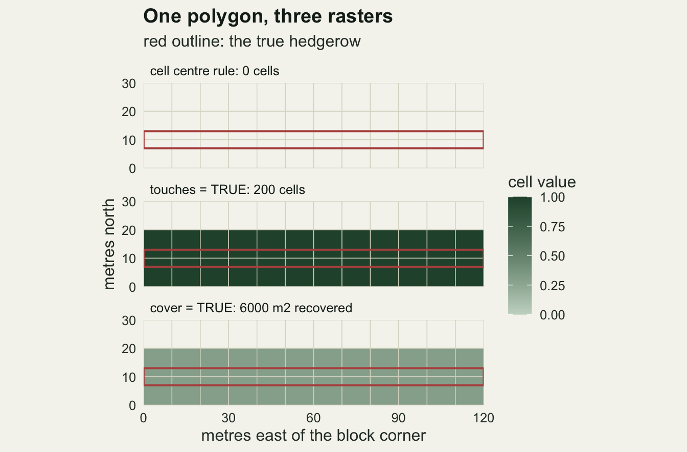
The overestimate is set by perimeter, not by area
A single strip is an extreme case, so the next step holds the habitat amount fixed and changes only the shape. Two families of landscape are built inside the same square kilometre block, each carrying the same habitat area: parallel bands of decreasing width, and square blocks of decreasing size. Both are rotated by a fixed angle so that no edge lines up with the grid, which would otherwise make the arithmetic come out exact by accident.
spin_angle <- 27 * pi / 180
spin_at <- function(polys) {
  rot <- matrix(c(cos(spin_angle), sin(spin_angle),
                  -sin(spin_angle), cos(spin_angle)), 2, 2)
  st_sf(id = seq_along(polys),
        geometry = st_sfc((st_sfc(polys) - c(500, 500)) * rot +
                            c(x_org + 750, y_org + 750), crs = utm))
}
bands_of <- function(wd) {
  n_band <- round(100 / wd); pitch <- 1000 / n_band
  spin_at(lapply(seq_len(n_band), function(i)
    box_of(50, 10 + pitch * (i - 1), 900, wd)))
}
blocks_of <- function(n_blk, side = 300 / sqrt(n_blk)) {
  k <- ceiling(sqrt(n_blk)); pitch <- (1000 - side) / max(k - 1, 1)
  ij <- expand.grid(i = 0:(k - 1), j = 0:(k - 1))[seq_len(n_blk), ]
  spin_at(lapply(seq_len(n_blk), function(q)
    box_of(ij$i[q] * pitch, ij$j[q] * pitch, side, side)))
}
land_r <- rast(xmin = x_org, xmax = x_org + 1500, ymin = y_org,
               ymax = y_org + 1500, resolution = cell_m, crs = utm)
score_of <- function(lay, fam) {
  vv <- vect(lay)
  edge <- st_length(st_cast(st_geometry(lay), "MULTILINESTRING"))
  data.frame(family = fam, peri = sum(as.numeric(edge)),
    truth = sum(as.numeric(st_area(lay))),
    centre = n_cells(rasterize(vv, land_r, field = 1)) * cell_m^2,
    touch = n_cells(rasterize(vv, land_r, field = 1, touches = TRUE)) * cell_m^2,
    cvr = sum_val(rasterize(vv, land_r, field = 1, cover = TRUE)) * cell_m^2)
}

band_w <- c(100, 50, 20, 10, 5, 2.5); blk_n <- c(1, 4, 16, 64, 256, 1024)
shape_tab <- rbind(
  do.call(rbind, lapply(band_w, function(wd) score_of(bands_of(wd), "bands"))),
  do.call(rbind, lapply(blk_n, function(nb) score_of(blocks_of(nb), "blocks"))))
shape_tab$narrow <- c(band_w, 300 / sqrt(blk_n))
shape_tab$err_t <- shape_tab$touch - shape_tab$truth
shape_tab$err_c <- shape_tab$centre - shape_tab$truth
print(with(shape_tab, data.frame(family, narrow_m = round(narrow, 3),
  perim_km = round(peri / 1000, 2), habitat_ha = truth / 1e4,
  touch_ha = round(touch / 1e4, 2), centre_ha = round(centre / 1e4, 2),
  cover_ha = round(cvr / 1e4, 4))), row.names = FALSE)
family narrow_m perim_km habitat_ha touch_ha centre_ha cover_ha
bands 100.000 2.0 9 10.39 8.96 8.9993
bands 50.000 3.8 9 11.61 8.97 8.9999
bands 20.000 9.2 9 15.29 8.95 8.9997
bands 10.000 18.2 9 21.38 8.96 8.9998
bands 5.000 36.2 9 33.55 9.00 8.9999
bands 2.500 72.2 9 57.95 9.00 8.9999
blocks 300.000 1.2 9 9.81 9.01 8.9997
blocks 150.000 2.4 9 10.68 8.96 8.9992
blocks 75.000 4.8 9 12.56 9.24 8.9996
blocks 37.500 9.6 9 16.04 8.80 9.0004
blocks 18.750 19.2 9 24.40 9.00 9.0004
blocks 9.375 38.4 9 45.20 8.96 8.9996pool_fit <- lm(err_t ~ 0 + peri, data = shape_tab)
pool_co <- summary(pool_fit)$coefficients / cell_m
fit_fam <- function(fam) summary(lm(err_t ~ 0 + peri,
data = shape_tab[shape_tab$family == fam, ]))$coefficients / cell_m
band_co <- fit_fam("bands"); blok_co <- fit_fam("blocks")
slope_geo <- (cos(spin_angle) + sin(spin_angle)) / 2
gap_of <- function(co) 100 * (co[1, 1] - slope_geo) / slope_geo
band_z <- (band_co[1, 1] - slope_geo) / band_co[1, 2]
pool_res <- 100 * (shape_tab$err_t - fitted(pool_fit)) / fitted(pool_fit)
band_res <- sort(abs(pool_res[shape_tab$family == "bands"]))
worst_i <- which.max(pool_res); spin_deg <- spin_angle * 180 / pi
hab_ha <- mean(shape_tab$truth) / 1e4; n_shape <- nrow(shape_tab)
peri_span <- range(shape_tab$peri) / 1000; err_span <- range(shape_tab$err_t) / 1e4
centre_rel <- 100 * shape_tab$err_c / shape_tab$truth
bnd_cells <- (shape_tab$touch - shape_tab$centre) / cell_m^2
miss_cells <- max(abs(shape_tab$err_c)) / cell_m^2
hab_cells <- mean(shape_tab$truth) / cell_m^2; fewest_i <- which.min(bnd_cells)
per_k <- shape_tab$err_t / (shape_tab$peri * cell_m)
band_k <- per_k[shape_tab$family == "bands"]; blok_k <- per_k[shape_tab$family == "blocks"]
blk1_gap <- 100 * (blok_k[1] - slope_geo) / slope_geo
se_ratio <- blok_co[1, 2] / band_co[1, 2]All 12 landscapes hold 9 hectares of habitat. Their perimeters run from 1.2 to 72.2 kilometres, and the area that touches = TRUE invents runs from 0.81 to 48.95 hectares in step with it. Regressing the overestimate on perimeter through the origin over all 12, then dividing by the cell size, gives 0.728 square metres of spurious habitat per metre of edge per metre of cell, with a standard error of 0.030.
There is a geometric prediction to hold that against. An edge crossing a square grid at angle a to the axes passes through about abs(cos(a)) + abs(sin(a)) cells per cell width, and on average half of each of those cells lies outside the polygon, so the expected overestimate is that quantity halved, times the perimeter, times the cell size. At 27 degrees that prediction is 0.6725. The pooled interval covers it, but the pooled fit is the wrong summary, because the residuals are not noise: every band landscape sits between 4.5 and 6.8 per cent below the fitted line while the finest block lattice sits 29.5 per cent above it. Fitting the two families separately splits them. The bands give 0.6782 with a standard error of 0.0004, which sits 0.85 per cent above the geometric prediction and 13.4 standard errors away from it. For a boundary made of long straight edges the derivation is an excellent approximation and not an identity: a gap of that size is nothing to an ecologist, and a separation of that many standard errors is far too large to be sampling noise. The blocks give 0.9033, 34.3 per cent above it, with a standard error 73 times the size of the bands’ one, 0.0313.
That larger error is the interesting half. Dividing each landscape’s invented area by its own perimeter, rather than fitting one line to all six, the bands hardly move: 0.695 for the widest band down to 0.678 for the narrowest, settling just above the geometric value and staying there. The blocks climb instead, from 0.675 for the single 300 metre block, 0.37 per cent above the geometric value, to 0.943 for the lattice whose blocks are smaller than a cell. So the block figure is not a second constant. It is the average of a quantity that rises as the boundary acquires corners and the features drop below the cell, which is why one number quoted for both families averages a law and a departure from it. Bregt et al. 1991 measured the same quantity on the soil map of the Netherlands, so this is a property of grids rather than of synthetic rectangles.
Against that, the cell centre rule behaves completely differently. Across the same 12 landscapes its error on total area stays between -2.2 and 2.7 per cent, and in cells rather than per cent it never misses by more than 24 of the 900 cells the habitat occupies. That miss does not grow with the number of boundary cells, which runs from 80 to 4895 across these landscapes: cells rounded up and cells rounded down cancel at either end of that range, and the landscape with the fewest boundary cells, the single 300 metre block, misses by 0.1 per cent. What the rule loses is not the total, and the last two sections are about what it loses instead.
blk_side <- c(150, 75, 37.5, 18.75); blk_cnt <- c(16, 32, 64, 128)
fixed_p <- do.call(rbind, Map(function(nb, side)
  score_of(blocks_of(nb, side), "fixed perimeter"), blk_cnt, blk_side))
fixed_p$err_t <- fixed_p$touch - fixed_p$truth
fixed_p$rel <- 100 * fixed_p$err_t / fixed_p$truth
print(with(fixed_p, data.frame(blocks = blk_cnt, side_m = blk_side,
  perim_km = round(peri / 1000, 3), habitat_ha = truth / 1e4,
  invented_ha = round(err_t / 1e4, 2), relative_pct = round(rel, 1))),
  row.names = FALSE)
blocks side_m perim_km habitat_ha invented_ha relative_pct
16 150.00 9.6 36.0 6.64 18.4
32 75.00 9.6 18.0 6.71 37.3
64 37.50 9.6 9.0 7.04 78.2
128 18.75 9.6 4.5 8.13 180.7fp_area <- range(fixed_p$truth) / 1e4; fp_err <- range(fixed_p$err_t) / 1e4
fp_ratio <- max(fixed_p$truth) / min(fixed_p$truth)
fp_peri <- unique(round(fixed_p$peri / 1000, 3))Holding the perimeter fixed instead makes the same point from the other side. Halving the side of a block and doubling the count leaves the total edge alone and halves the area, so these four lattices all carry 9.6 kilometres of boundary while their habitat runs from 4.5 to 36.0 hectares, a factor of 8. The invented area barely moves with them: 6.64 to 8.13 hectares. As a share of the truth that is 18 per cent for the coarse lattice and 181 per cent for the fine one. Two landscape studies reporting the same habitat percentage can therefore be reporting quite different things, and the divergence is governed by how much edge each landscape has, which is the quantity fragmentation studies treat as a result rather than as a nuisance.
fam_line <- data.frame(family = c("bands", "blocks"), icpt = 0,
                       slope = c(band_co[1, 1], blok_co[1, 1]) * cell_m / 10)
ggplot(shape_tab, aes(peri / 1000, err_t / 1e4)) +
  geom_abline(data = fam_line,
              aes(slope = slope, intercept = icpt, colour = family),
              linetype = "dashed", linewidth = 0.6) +
  geom_point(data = fixed_p, aes(peri / 1000, err_t / 1e4),
             colour = te_ink, shape = 0, size = 3.6, stroke = 0.9) +
  geom_point(aes(colour = family, shape = family), size = 2.6) +
  annotate("text", x = 12.5, y = 6.4, hjust = 0, size = 3.4, colour = te_ink,
           label = "one perimeter, four lattices, eightfold range of area") +
  scale_colour_manual(values = c(bands = te_forest, blocks = te_gold),
                      name = NULL) +
  scale_shape_manual(values = c(bands = 16, blocks = 17), name = NULL) +
  labs(x = "perimeter (km)", y = "invented habitat (ha)",
       title = "The overestimate follows the edge, at two rates",
       subtitle = "dashed: origin fit within each family") +
  theme_datasheet() + theme(legend.position = "bottom")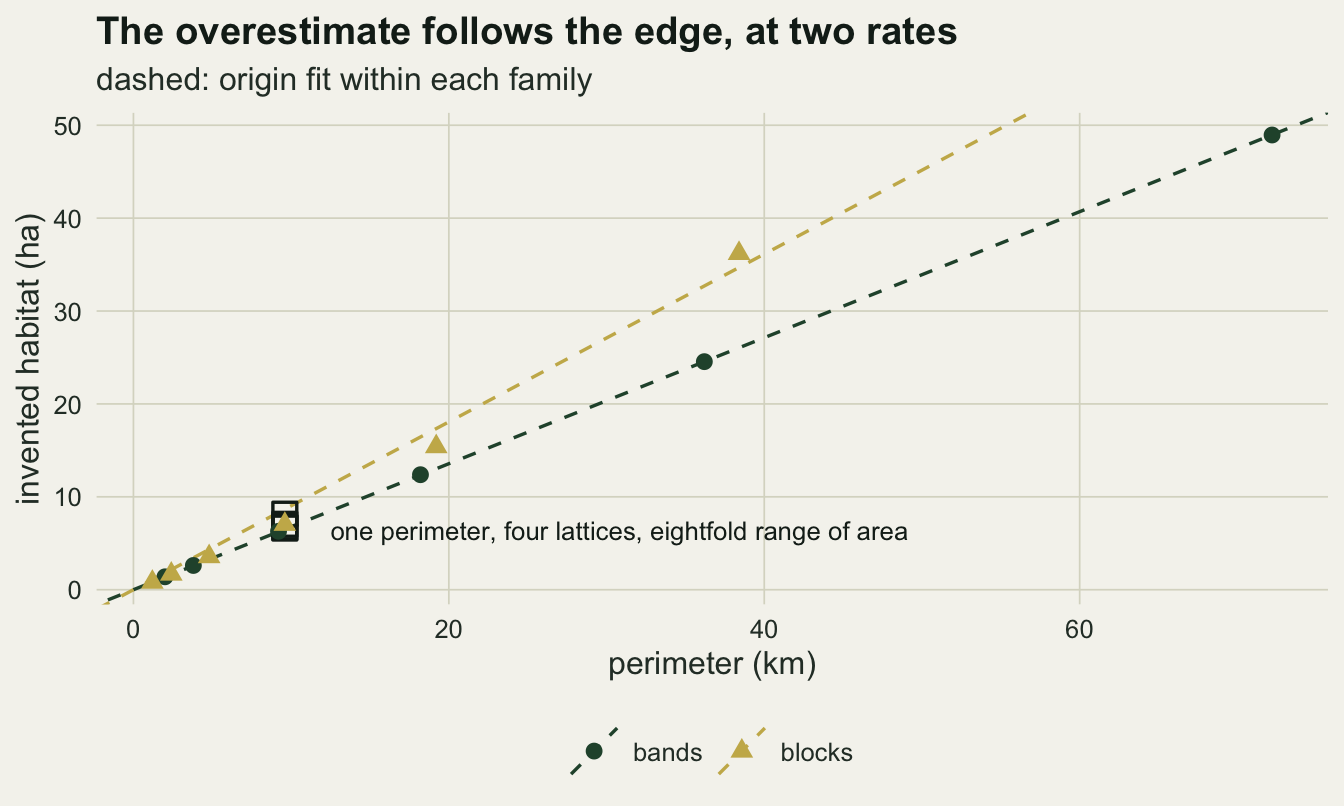
How fine the grid has to be before the rule stops mattering
The practical question is what cell size makes the choice irrelevant. Sweeping the cell size under the same hedgerow answers it, but the cell centre rule needs replication, because its answer depends on where the grid origin happens to fall. Twenty grid origins per cell size were fixed before any of these numbers were seen, and the Monte Carlo error on each mean is the standard deviation across origins divided by the square root of twenty. The origin is shifted in both directions and the raster is sized to cover the whole strip at every cell size: a grid whose column count does not divide the length of the strip clips the last part of it, and that clip is a property of the extent rather than of the rule.
n_origin <- 20; set.seed(2262)
sh_x <- runif(n_origin, 0, cell_m); sh_y <- runif(n_origin, 0, cell_m)
grain_tab <- do.call(rbind, lapply(c(10, 5, 3, 2, 1.2, 0.6, 0.3), function(dd) {
  got <- vapply(seq_len(n_origin), function(k) {
    xa <- x_org - sh_x[k]; ya <- y_org - sh_y[k]
    nc <- ceiling((strip_len + sh_x[k]) / dd) + 1
    nr <- ceiling((strip_h + sh_y[k]) / dd) + 1
    fine_r <- rast(xmin = xa, xmax = xa + nc * dd, ymin = ya,
                   ymax = ya + nr * dd, ncols = nc, nrows = nr, crs = utm)
    c(n_cells(rasterize(hedge_v, fine_r, field = 1)) * dd^2,
      n_cells(rasterize(hedge_v, fine_r, field = 1, touches = TRUE)) * dd^2)
  }, numeric(2))
  data.frame(d_m = dd, ratio = dd / strip_w, centre_mean = mean(got[1, ]),
             centre_sd = sd(got[1, ]), touch_mean = mean(got[2, ]),
             touch_sd = sd(got[2, ]))
}))
pct_of <- function(v) 100 * (v - strip_area) / strip_area
grain_tab$centre_pct <- pct_of(grain_tab$centre_mean)
grain_tab$spread_pct <- 100 * grain_tab$centre_sd / strip_area
grain_tab$mc_pct <- grain_tab$spread_pct / sqrt(n_origin)
grain_tab$touch_pct <- pct_of(grain_tab$touch_mean)
grain_tab$touch_mc <- 100 * grain_tab$touch_sd / strip_area / sqrt(n_origin)
print(round(grain_tab[, c("d_m", "ratio", "centre_pct", "mc_pct", "spread_pct",
                          "touch_pct", "touch_mc")], 3), row.names = FALSE)
d_m ratio centre_pct mc_pct spread_pct touch_pct touch_mc
10.0 1.667 16.667 17.522 78.360 160.917 19.212
5.0 0.833 0.000 7.647 34.199 88.438 8.320
3.0 0.500 0.035 0.034 0.153 50.390 0.041
2.0 0.333 0.000 0.000 0.000 33.600 0.000
1.2 0.200 -0.004 0.013 0.056 20.146 0.016
0.6 0.100 -0.004 0.007 0.030 10.065 0.007
0.3 0.050 0.000 0.003 0.015 5.029 0.003near_row <- function(target) grain_tab[which.min(abs(grain_tab$ratio - target)), ]
coarse <- grain_tab[which.max(grain_tab$ratio), ]; moves <- grain_tab$centre_sd > 0
bias_z <- max(abs(grain_tab$centre_pct[moves] / grain_tab$mc_pct[moves]))
still_d <- grain_tab$d_m[!moves]
half_row <- near_row(0.5); ten_row <- near_row(0.1); five_row <- near_row(0.05)Two different failures come out of this. The cell centre rule shows no bias at any cell size once the grid is allowed to move under the strip: across every cell size whose answer moves with the origin at all, the largest gap between the mean and the truth is 1.02 Monte Carlo errors, and at 2 metre cells, where the strip is a whole number of cells wide and long, it is exact. At 10 metre cells that mean is 7000 square metres against a truth of 6000, but the Monte Carlo error on it is 17.5 per cent of the truth, so twenty origins say nothing sharper than that. It is the spread that is unusable: the standard deviation across origins is 78 per cent of the true area, and the alignment table shows why: at this cell size a single map returns either nothing or 10000 square metres, never the true 6000. That spread does collapse at the finer cell sizes here, to 0.15 per cent at a ratio of 0.50, but that is commensurability and not a threshold: every cell size in the sweep from 3 metres down divides the 6 metre width exactly, so only the two ends of the strip are left to round. On a cell that does not divide the width, one row of cells is in doubt at every alignment, and that row is the ratio’s share of the strip, so the spread falls with the ratio instead of switching off at half the width.
The touches rule needs a much finer grid, because its error is a bias rather than a spread: it comes down in proportion to the cell size and it does not cancel across features. Its relative overestimate stays close to the ratio of cell size to feature width throughout: 10.1 per cent at a ratio of 0.10, and 5.0 per cent at 0.05. The working rule of thumb is therefore a cell no larger than a tenth of the narrowest feature for ten per cent accuracy on area, and a twentieth for five per cent. For a 6 metre hedgerow that means a 0.6 metre grid, which over any real study area is an expensive raster.
Shape is a second caveat, and the sweep above is the easy case for it. This hedgerow is a straight rectangle whose edges run along the grid, so at a ratio of 0.05 the spread is down to 0.015 per cent. A boundary that cuts across the grid rounds at every cell along it, and a crenulated one rounds more often again. The rotated landscapes above are the first of those and not the second, since every polygon in them is a rectangle, and on single grid origins at 10 metre cells they still missed the total by between -2.2 and 2.7 per cent. Turner et al. 1989 made the general version of the point for landscape pattern: the grain sets which patterns are visible at all, and no metric computed on the grid can recover what the grain removed.
Coverage fraction gets the area right and gives up the patches
terra::rasterize() takes cover = TRUE, which returns the fraction of each cell covered by the polygon instead of a presence flag. Summed and multiplied by the cell area it is an area estimate, and on every landscape above it was right to a rounding error. It is worth knowing how it does that, because the help page says the fraction is estimated from at least 100 sub-cells, and that is a promise with a floor under it.
cvr_tab <- do.call(rbind, lapply(c(6, 5.5, 3.7, 2, 1.2, 0.5, 0.2), function(wd) {
  hv <- vect(one_of(x_org, y_org + 7, strip_len, wd))
  data.frame(width_m = wd, truth_m2 = strip_len * wd,
    cover_m2 = sum_val(rz(hv, cover = TRUE)) * cell_m^2,
    exact_m2 = sum_val(rasterizeGeom(hv, hedge_r, fun = "area")))
}))
cvr_tab$cover_pct <- 100 * (cvr_tab$cover_m2 - cvr_tab$truth_m2) / cvr_tab$truth_m2
print(round(cvr_tab, 2), row.names = FALSE)
width_m truth_m2 cover_m2 exact_m2 cover_pct
6.0 6000 6000 6000 0.00
5.5 5500 6000 5500 9.09
3.7 3700 4000 3700 8.11
2.0 2000 2000 2000 0.00
1.2 1200 1000 1200 -16.67
0.5 500 1000 500 100.00
0.2 200 0 200 -100.00cvr_step <- cell_m / 10; worst_row <- cvr_tab[which.max(cvr_tab$cover_pct), ]
gone_row <- cvr_tab[which.min(cvr_tab$width_m), ]
exact_err <- max(abs(cvr_tab$exact_m2 - cvr_tab$truth_m2))
probe_len <- 200; probe_w <- gone_row$width_m; probe_col <- c(20, 60, 100)
probe_v <- vect(one_of(x_org, y_org + 7, probe_len, probe_w))
probe <- vapply(probe_col, function(nc) {
pr <- rast(xmin = x_org, xmax = x_org + nc * cell_m, ymin = y_org,
ymax = y_org + strip_h, resolution = cell_m, crs = utm)
vv <- values(rasterize(probe_v, pr, field = 1, cover = TRUE))
if (all(is.na(vv))) 0 else max(vv, na.rm = TRUE)
}, numeric(1))
probe_n <- probe_col * strip_h / cell_m; probe_truth <- probe_w / cell_mThe coverage column moves in steps: every estimate is a multiple of 1.0 metres of width, because a ten by ten subgrid is what 100 sub-cells buys and each sub-cell is tested by its own centre. Coverage fraction is the cell centre rule applied at a tenth of the grain, which is why it is unbiased and far less noisy, and also why it drops out here. At 0.5 metres wide it is out by 100 per cent, and at 0.2 metres it returns 0: the strip has disappeared again. This is the floor a minimum mapping unit imposes on a classified land cover product, whose effect on composition and configuration Saura 2002 quantified.
The tenth of a cell is a floor and not a fixed sub-cell size, though, and it is worth knowing which side of it a given raster falls on. The help page says at least 100 sub-cells, more if there are very few cells, and it means it. The same 0.2 metre strip, 200 metres long, on the same 10 metre cells, returns 0.0200 on a raster of 60 cells, 0.0625 on one of 180, and 0.0000 on one of 300, against a true fraction of 0.0200. A small raster gets a finer subgrid, which here happens to land on the truth once and to overshoot it once; only from a few hundred cells up does the tenth-of-a-cell quantisation bind, and every raster in this post is on that side of the line.
Against that floor, terra::rasterizeGeom(v, r, fun = "area") has none. It computes the geometric intersection of each polygon with each cell and returns the area, and across the whole width sweep it reproduces the true area with a largest absolute error of 0.0000 square metres. If the number you want is habitat area, that is the function to use. The price of both area-preserving methods is the same, though, and it is not small. Neither output is a habitat map. A coverage raster holds a number between zero and one in every cell near a boundary, so there is no such thing as a patch in it: no connected component to label, no adjacency to count, no edge to measure. Anything that needs discrete habitat has to threshold it, and a threshold is a third rule with its own arbitrariness.
tiny <- blocks_of(1024); tiny_v <- vect(tiny); tiny_n <- nrow(tiny)
tiny_true <- sum(as.numeric(st_area(tiny))); tiny_side <- sqrt(as.numeric(st_area(tiny))[1])
hit <- table(values(rasterize(tiny_v, land_r, field = "id", fun = "min")))
got <- integer(tiny_n); got[as.integer(names(hit))] <- as.integer(hit)
lost_n <- sum(got == 0); lost_pct <- 100 * mean(got == 0)
tot_pct <- 100 * sum(got) * cell_m^2 / tiny_true
tiny_touch <- rasterize(tiny_v, land_r, field = 1, touches = TRUE)
tiny_ratio <- n_cells(tiny_touch) * cell_m^2 / tiny_true
tiny_cell <- st_as_sf(as.polygons(tiny_touch, dissolve = FALSE))
tiny_hit <- lengths(st_intersects(tiny, tiny_cell)); tiny_keep <- sum(tiny_hit > 0)
The gap between getting the total right and getting the features right is easiest to see in the lattice of 1024 blocks, each 9.375 metres across and so smaller than one cell. Under the cell centre rule the total area comes out at 99.6 per cent of the truth, which any reviewer would wave through, while 140 of the 1024 blocks, 14 per cent of them, are not in the raster at all. The total holds up because the blocks that did survive were rounded up by as much as the vanished ones were rounded down. Under touches = TRUE all 1024 blocks survive, which is a certainty rather than a discovery because the cells tile the plane, and the cost of that certainty is the count: each block lands in between 3 and 6 cells, a mean of 4.41, so the habitat area comes out 5.0 times the truth.
The patch count inherits the rule
The last step is to push each raster into something ecological. The layer here is a small woodland network: four blocks joined by hedgerows six metres wide, and a separate cluster of nine small woods with seven metre gaps between them. As vector geometry the truth is not in doubt.
blocks4 <- lapply(0:3, function(i)
  box_of(x_org + 82 + 180 * i, y_org + 202, 120, 120))
links3 <- lapply(0:2, function(i)
  box_of(x_org + 202 + 180 * i, y_org + 257, 60, strip_w))
cluster9 <- lapply(0:8, function(q)
  box_of(x_org + 852 + 47 * (q %% 3), y_org + 202 + 47 * (q %/% 3), 40, 40))
netw <- st_sf(id = seq_len(16),
              geometry = st_sfc(c(blocks4, links3, cluster9), crs = utm))
comp_a <- as.numeric(st_area(st_cast(st_union(netw), "POLYGON")))
true_n <- length(comp_a); true_area <- sum(comp_a)
true_lpi <- max(comp_a) / true_area
link_share <- 100 * sum(as.numeric(st_area(st_sfc(links3, crs = utm)))) / true_area
netw_r <- rast(xmin = x_org, xmax = x_org + 1100, ymin = y_org,
               ymax = y_org + 450, resolution = cell_m, crs = utm)
netw_v <- vect(netw)
metrics_of <- function(rst) {
  szs <- as.vector(table(values(patches(rst, directions = 4))))
  c(area_ha = n_cells(rst) * cell_m^2 / 1e4, patches = length(szs),
    lpi = max(szs) / sum(szs))
}
r_centre <- rasterize(netw_v, netw_r, field = 1)
r_touch <- rasterize(netw_v, netw_r, field = 1, touches = TRUE)
r_cvr <- rasterize(netw_v, netw_r, field = 1, cover = TRUE)
m_c <- metrics_of(r_centre); m_t <- metrics_of(r_touch)
m_m <- metrics_of(ifel(r_cvr >= 0.5, 1, NA))
truth_row <- c(area_ha = true_area / 1e4, patches = true_n, lpi = true_lpi)
print(round(rbind(truth = truth_row, cell_centre = m_c, touches = m_t,
                  cover_over_half = m_m), 3))
area_ha patches lpi
truth 7.308 10 0.803
cell_centre 7.200 13 0.200
touches 9.020 2 0.783
cover_over_half 7.170 13 0.201cvr_area_ha <- sum_val(r_cvr) * cell_m^2 / 1e4; cvr_gap <- abs(cvr_area_ha * 1e4 - true_area)
link_cvr <- rasterize(vect(st_sf(id = 1:3, geometry = st_sfc(links3, crs = utm))),
netw_r, field = 1, cover = TRUE)
link_fill <- 100 * max(values(link_cvr), na.rm = TRUE)The vector layer contains 10 connected components: one chain and nine isolated woods. The hedgerows that make the chain a chain are 1.48 per cent of the habitat area, so they are invisible in any summary of habitat amount, and they carry all of the connectivity. The cell centre rule loses them and returns 13 patches, with the largest holding 20.0 per cent of the habitat against a true 80.3 per cent. The touches rule keeps the hedgerows, but it also bridges the seven metre gaps in the cluster, fusing nine woods into one, and returns 2 patches with a largest patch index of 78.3 per cent. One rule says this landscape is shattered, the other says it is almost entirely connected, and the vector layer says neither: its largest patch index sits near the touches figure, so what touches gets wrong is the count, while the cell centre rule gets the count and the share wrong.
Coverage fraction recovers the habitat area to within 0.0023 square metres, 7.3080 hectares against 7.3080, and answers none of the questions above. That near-exactness is partly luck: every edge in this network sits on a whole metre, which is a boundary of the tenth-of-a-cell subgrid, so no sub-cell has to be resolved half in and half out. A layer digitised off an aerial photograph would not oblige. Thresholding it at half a cell, which is the majority rule the fragmentation post applies to a raster that already exists, returns 13 patches. Because each hedgerow straddles a row boundary it fills at most 30 per cent of any one cell, so the majority rule discards it exactly as the cell centre rule did.
patch_df <- function(rst, lab) {
  pl <- patches(rst, directions = 4); szs <- table(values(pl))
  dd <- as.data.frame(pl, xy = TRUE); names(dd)[3] <- "pid"
  dd$size_ha <- as.numeric(szs[as.character(dd$pid)]) * cell_m^2 / 1e4
  dd$x <- dd$x - x_org; dd$y <- dd$y - y_org; dd$rule <- lab; dd
}
net_long <- rbind(
  patch_df(r_centre, sprintf("cell centre rule: %.0f patches", m_c[["patches"]])),
  patch_df(r_touch, sprintf("touches = TRUE: %.0f patches", m_t[["patches"]])))
ggplot(net_long, aes(x, y, fill = size_ha)) +
  geom_tile(width = cell_m, height = cell_m) +
  facet_wrap(~rule, ncol = 1) + coord_equal(expand = FALSE) +
  scale_fill_gradient(low = "#cfdccf", high = te_forest,
                      name = "patch size (ha)") +
  labs(x = "metres east", y = "metres north",
       title = "One layer, two landscapes",
       subtitle = "identical vector input, identical grid") +
  theme_datasheet() +
  theme(panel.grid = element_blank(),
        strip.text = element_text(colour = te_ink, hjust = 0))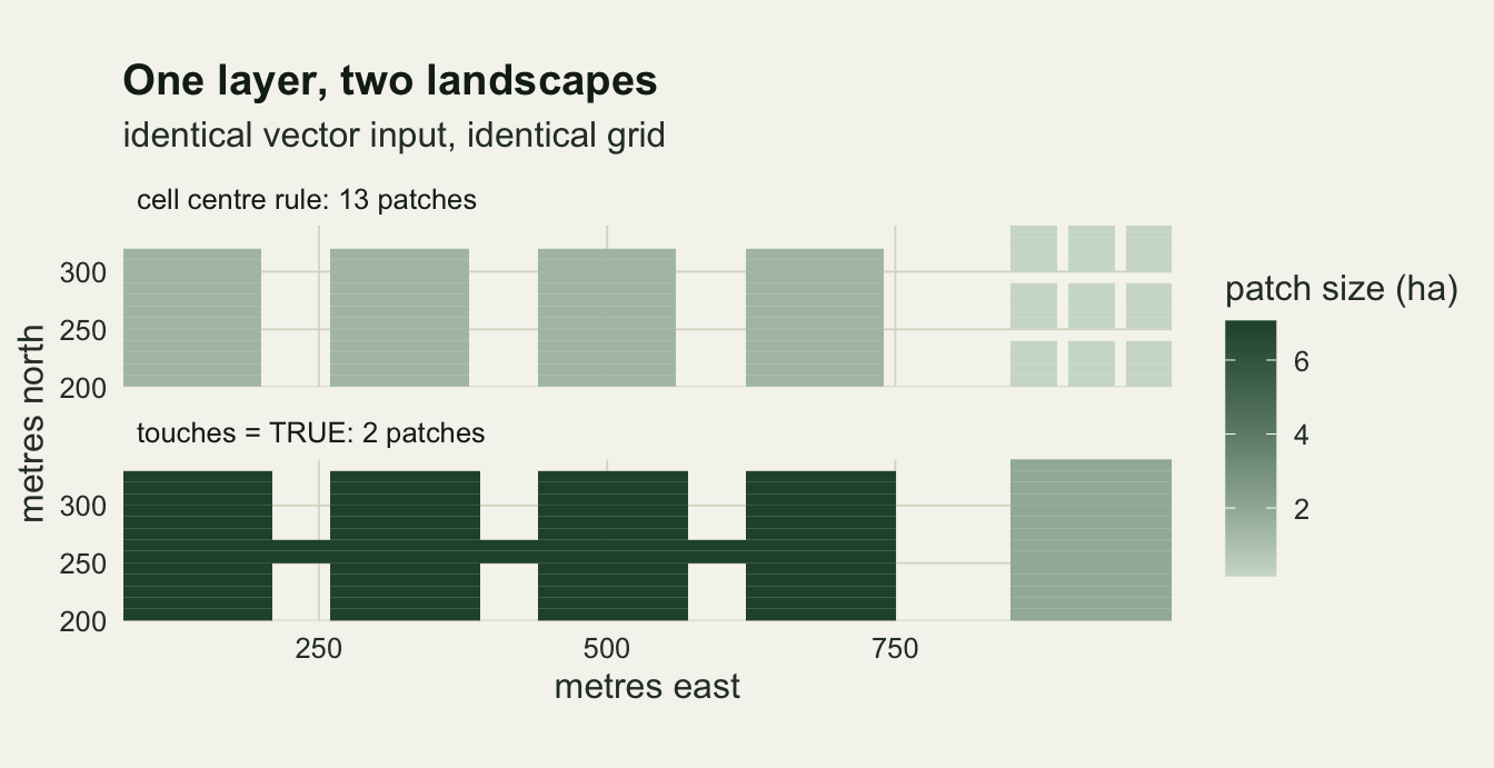
What to report
Say which rasterisation rule produced the habitat layer. In terra that means saying whether touches was left at its default or set to TRUE; in QGIS or GDAL it means saying whether ALL_TOUCHED was on. They are different measurements of the same landscape, and on the hedgerow above there is no factor that converts one into the other: the default returned 0 square metres and ALL_TOUCHED returned 20000, against a truth of 6000. Only the second can be expressed as a ratio to the truth, and it is 3.33.
Give the cell size next to the width of the narrowest feature the analysis cares about. A cell size on its own is not interpretable; the ratio is. Anything above about a tenth is a warning that the area figure carries a bias of roughly that ratio if touches was on, and a lottery of comparable size if it was not.
If the quantity of interest is area, do not take it from a presence raster at all. Compute it on the vector layer with st_area, or with rasterizeGeom(..., fun = "area") if it has to be resolved per cell. Rasterise for the things that need a grid and keep the area from the geometry. If the quantity of interest is patches, connectivity or edge, say so and accept that the rule is now part of the result. Report the patch count under both rules whenever the features carrying the connectivity are narrow, because a corridor network is precisely the case where the two answers are furthest apart. Report the coordinate reference system and the grid origin too, not only the resolution: two rasters covering the same area at the same resolution but with different origins give different maps of the same narrow features, which the alignment table shows directly.
Honest limits
Every polygon here is a rectangle, and rectangles have a perimeter that is easy to reason about. Real habitat polygons have crenulated boundaries whose measured perimeter depends on the digitising scale, so the perimeter that drives the error is not a fixed property of the landscape either. Of the two constants, only the band one, 0.678, behaves like a constant; the block figure of 0.903 averages a per-landscape quantity that runs from 0.675 to 0.943 and is still rising at the finest lattice, so it is a summary of this particular ladder of block sizes and not a number to multiply by a perimeter taken from some other source. Each family also carries only 6 landscapes, which is thin for a slope: the block standard error alone is 0.031.
All the landscapes were rotated by one angle, 27 degrees, and the geometric prediction depends on that angle: it is smallest for edges parallel to the grid and largest at 45 degrees. A landscape with a dominant field orientation aligned to the grid, which happens whenever the grid was built from an aerial survey flown along the field pattern, sits below the line drawn here. A second geometric assumption sits beside that one: the exact area from rasterizeGeom is exact in the plane, not on the ellipsoid. On a projected grid in metres over a small block that distinction does not matter; on a geographic grid it does, because cell areas vary with latitude, and the sums above would need weighting before they meant anything.
The cell centre rule is described here as unbiased for total area, and that holds because a cell centre is as likely to fall inside a boundary that ought to have excluded it as outside one that ought to have taken it in. It is a poor description of a single feature: the hedgerow section shows one polygon whose measured area was zero, and the sub-cell lattice shows 14 per cent of features lost while the total came in only 0.4 per cent short. A study reporting a landscape total is protected by that cancellation. A study reporting anything per feature is not.
The connectivity example uses four-neighbour connectivity throughout. Switching to eight neighbours would reconnect some of what the cell centre rule broke, and would merge still more of what touches had already merged, so the patch counts quoted are specific to that choice as well as to the rasterisation rule. Two independent conventions are stacked inside a single reported number.
References
Bregt AK, Denneboom J, Gesink HJ, van Randen Y 1991 International Journal of Geographical Information Systems 5(3):361-367 (10.1080/02693799108927861)
Turner MG, O’Neill RV, Gardner RH, Milne BT 1989 Landscape Ecology 3(3-4):153-162 (10.1007/BF00131534)
Jelinski DE, Wu J 1996 Landscape Ecology 11(3):129-140 (10.1007/BF02447512)
Saura S 2002 International Journal of Remote Sensing 23(22):4853-4880 (10.1080/01431160110114493)
Davies ZG, Pullin AS 2007 Landscape Ecology 22(3):333-351 (10.1007/s10980-006-9064-4)
Hijmans RJ 2023 terra: Spatial Data Analysis. R package version 1.7-65 (https://CRAN.R-project.org/package=terra)