library(terra)
library(ggplot2)
terraOptions(progress = 0)

te_paper  <- "#f5f4ee"; te_ink    <- "#16241d"; te_body   <- "#2c3a31"
te_forest <- "#275139"; te_rust   <- "#b5534e"; te_gold   <- "#c9b458"
te_line   <- "#dad9ca"

theme_datasheet <- function() theme_minimal(base_size = 12) +
  theme(plot.background = element_rect(fill = te_paper, colour = NA),
        panel.background = element_rect(fill = te_paper, colour = NA),
        panel.grid.major = element_line(colour = te_line, linewidth = 0.3),
        panel.grid.minor = element_blank(), text = element_text(colour = te_body),
        plot.title = element_text(colour = te_ink, face = "bold"),
        plot.subtitle = element_text(colour = te_body), axis.text = element_text(colour = te_body))
class_col <- c(water = "#5b8aa6", wetland = "#8fb3a3", grassland = te_gold,
               scrub = te_rust, forest = te_forest)
terra_ver <- as.character(packageVersion("terra")); gdal_r <- gdal(); proj_r <- gdal(lib = "proj")
qgis_ver  <- "3.34.4"; gdal_q <- "3.8.4"; proj_q <- "9.4.0"   # qgis_process --version, where the files were made
n_cells <- function(n) sprintf("%d %s", n, if (n == 1) "cell" else "cells")Reprojecting a raster in QGIS and R: opposite defaults
R
QGIS
terra
GIS
spatial
raster data
ecology tutorial
QGIS Warp copies the nearest cell and terra project() interpolates unless told otherwise. What each does to a land-cover map and a DEM, and how to match them.
A land-cover map classified from Landsat scenes arrives in UTM zone 34 north, the zone the scenes were delivered in. The protected-area boundaries and the national grid it has to be reported on are in Stereo70 (EPSG:3844), the Romanian national system, so the map is reprojected: once in QGIS, to look at it over the other layers, and once in R with terra, for the analysis. The two versions disagree along the patch boundaries, and the R version holds class codes that are not whole numbers. A digital elevation model goes through the same step, and the slope map made from one of its two versions is crossed by a lattice of faint straight lines. Nothing failed. The two programs resampled the cells in different ways, and neither said which.
Every reprojection of a raster builds a new grid in the new coordinate system and has to decide what value each new cell takes from the old ones. Rasterising a vector layer measures the rule that decides which cells a polygon fills; this post is the rule one step later, when a grid becomes another grid. Checking a remote sensing covariate compares the nearest pixel and bilinear interpolation as ways of reading a satellite image at survey stations; the same two rules are at work here, applied to every cell of the output. Which coordinate system to choose in the first place is the subject of Choosing a projection for area and distance, and is not repeated. Raster data in R with terra is the place to start if a SpatRaster is new to you. Like Area in QGIS and R, the page has no screenshots: menu paths are in bold, the QGIS commands are shown exactly as they ran, and the R chunks read their output rasters back from this post’s folder.
The short answer
The two tools make opposite choices when you do not choose. QGIS Raster > Projections > Warp (Reproject) copies the value of the nearest old cell into each new cell. terra::project() interpolates between the four nearest old cells, unless the raster has a category table (or is an RGB image), in which case it copies the nearest one too. A land-cover GeoTIFF of plain integer codes, with no category names or attribute table stored in the file or beside it (a colour table alone does not count), is not a factor, so terra averages the codes: along every boundary it writes values between classes, and after rounding some of those are classes that were never there. For a map of classes, pass method = "near" to project(), or give the raster its category table with levels() first; QGIS needs nothing. For an elevation or temperature surface the choice is the other way round: bilinear keeps the shape of the surface but cuts the top off sharp peaks, while nearest keeps every value but moves some of them, and slope computed from the result shows it. Choose Bilinear (2x2 Kernel) in the Warp dialog, or leave terra on its default. Both tools pick the output cell size on their own, and they pick the same one; to control the grid, give both the same template.
| In QGIS (Warp) | In R (terra) |
What happens |
|---|---|---|
Resampling method to use left at Nearest Neighbour |
project(x, "EPSG:3844", method = "near") |
each new cell copies one old cell |
Resampling method to use set to Bilinear (2x2 Kernel) |
project(x, "EPSG:3844") on a raster with no category table |
each new cell is a weighted mean of four old cells |
| (the QGIS default) | project(x, "EPSG:3844") after levels(x) <- ... |
nearest cell, and the output keeps the categories |
Output data type (under Advanced Parameters) left at Use Input Layer Data Type |
no equivalent: bilinear output is floating point | QGIS rounds bilinear values back into the input’s integer type |
| Output file resolution in target georeferenced units | project(x, "EPSG:3844", res = 30) |
same cell size, grids anchored at different corners |
| Georeferenced extents plus resolution | project(x, template) |
the same grid in both, cell for cell |
| Layer Properties > Symbology, Resampling | none: it changes the screen, not the file | display only; nearest neighbour unless changed, according to the QGIS source |
The sections below measure each row.
Two rasters, written by R
Both inputs are synthetic and sit in UTM zone 34 north, in a block of Transylvania. The land-cover map is 200 by 200 cells of 30 metres. Its patches are the areas closest to 70 random centres, and each patch gets one of five class codes at random: 1 water, 2 wetland, 3 grassland, 4 scrub, 5 forest. The codes are labels, not quantities, and because they are assigned at random, water often borders forest, which is what a real classification does too. The elevation model is 120 by 120 cells of 30 metres over part of the same block: a broad hill, a small conical knoll 30 metres high and 120 metres in radius, a gentle tilt to the east and half a metre of noise. The chunk writes both as GeoTIFFs next to this page, and those two files are the input to every QGIS command below.
utm <- "EPSG:32634"; stereo <- "EPSG:3844"
block <- rast(nrows = 200, ncols = 200, xmin = 650000, xmax = 656000,
              ymin = 5176000, ymax = 5182000, crs = utm)
block_xy <- xyFromCell(block, seq_len(ncell(block)))
voronoi_cover <- function(n_patch) {   # patches around random centres, random class codes
  px <- runif(n_patch, 650000, 656000); py <- runif(n_patch, 5176000, 5182000)
  code <- sample(1:5, n_patch, replace = TRUE)
  nearest <- integer(nrow(block_xy))
  for (b in split(seq_len(nrow(block_xy)), ceiling(seq_len(nrow(block_xy)) / 2000))) {
    d2 <- outer(block_xy[b, 1], px, "-")^2 + outer(block_xy[b, 2], py, "-")^2
    nearest[b] <- max.col(-d2, ties.method = "first")
  }
  setValues(block, code[nearest])
}
set.seed(20261012)
cover_made <- voronoi_cover(70); names(cover_made) <- "cover"
writeRaster(cover_made, "landcover-utm.tif", overwrite = TRUE, datatype = "INT1U",
            gdal = "COMPRESS=DEFLATE")
cover <- rast("landcover-utm.tif")
classes <- c("water", "wetland", "grassland", "scrub", "forest")

hill_xy <- c(652260, 5179160); knoll_xy <- c(653590, 5178080)
surface <- function(x, y) {            # the elevation model without its noise, metres
  420 + 180 * exp(-((x - hill_xy[1])^2 + (y - hill_xy[2])^2) / (2 * 650^2)) +
    30 * pmax(0, 1 - sqrt((x - knoll_xy[1])^2 + (y - knoll_xy[2])^2) / 120) +
    40 * (x - 651000) / 3600
}
set.seed(20261013)
dem_grid <- rast(nrows = 120, ncols = 120, xmin = 651000, xmax = 654600,
                 ymin = 5177000, ymax = 5180600, crs = utm)
dem_xy   <- xyFromCell(dem_grid, seq_len(ncell(dem_grid)))
dem_made <- setValues(dem_grid, surface(dem_xy[, 1], dem_xy[, 2]) +
                        rnorm(ncell(dem_grid), 0, 0.5))
names(dem_made) <- "elevation"
writeRaster(dem_made, "dem-utm.tif", overwrite = TRUE, datatype = "FLT4S",
            gdal = c("COMPRESS=DEFLATE", "PREDICTOR=3"))
dem <- rast("dem-utm.tif")
cover_share <- prop.table(table(factor(values(cover)[, 1], levels = 1:5)))
Two tools, two defaults
In QGIS the tool is Raster > Projections > Warp (Reproject), which is the GDAL gdalwarp program behind a dialog, gdal:warpreproject in the Processing toolbox. Its Resampling method to use starts at Nearest Neighbour, and qgis_process help gdal:warpreproject prints the same thing: RESAMPLING, default value 0, and 0 is Nearest Neighbour. The commands below ran once each against QGIS 3.34.4 on Linux, in this post’s folder. The first is the default, the second asks for bilinear, and the rest are used further down. OPTIONS=COMPRESS=DEFLATE only compresses the files and does not change a value. On this build each run starts with two lines reading ERROR: Status 2: File EPSG:3844 could not be found and then completes normally; the outputs were not affected.
export QT_QPA_PLATFORM=offscreen
warp() {  # input, output, then any extra parameters
  qgis_process run gdal:warpreproject -- INPUT="$1" TARGET_CRS=EPSG:3844 \
    OPTIONS=COMPRESS=DEFLATE OUTPUT="$2" "${@:3}"
}
warp landcover-utm.tif qgis-landcover-near.tif
warp landcover-utm.tif qgis-landcover-bilinear.tif RESAMPLING=1
warp landcover-utm.tif qgis-landcover-exact.tif EXTRA="-et 0"
warp landcover-utm.tif qgis-landcover-bilinear-exact.tif RESAMPLING=1 EXTRA="-et 0"
warp landcover-utm.tif qgis-landcover-res30.tif TARGET_RESOLUTION=30
warp landcover-utm.tif qgis-landcover-template.tif TARGET_RESOLUTION=30 \
  TARGET_EXTENT="344400,350730,581820,588150 [EPSG:3844]"
warp dem-utm.tif qgis-dem-near.tif
warp dem-utm.tif qgis-dem-bilinear.tif RESAMPLING=1
In terra, project() chooses when method is not given. The rule is two lines in the package source: if the raster is a factor, that is, has a category table, or is flagged as an RGB image, the method is "near", and otherwise it is "bilinear". rast() makes a factor only when the file carries category names or a raster attribute table, inside the GeoTIFF or beside it in a .tif.aux.xml or .vat.dbf file. A colour table alone does not count (and bilinear output drops it). The land-cover file here has none of these.
cover_is_factor <- is.factor(cover)
t_default <- project(cover, stereo)                   # terra, no method given
t_near    <- project(cover, stereo, method = "near")
q_near    <- rast("qgis-landcover-near.tif")          # QGIS, no method given
q_bil     <- rast("qgis-landcover-bilinear.tif")
q_exact   <- rast("qgis-landcover-exact.tif")
q_bil_ex  <- rast("qgis-landcover-bilinear-exact.tif")
td <- values(t_default)[, 1]; ok <- !is.na(td)
non_int   <- mean(td[ok] != round(td[ok]))
same_grid <- isTRUE(all.equal(as.vector(ext(q_near)), as.vector(ext(t_default)))) &&
  all(dim(q_near) == dim(t_default))
n_out     <- sum(ok)
diff_near  <- sum(values(q_near)[, 1] != values(t_near)[, 1], na.rm = TRUE)
diff_exact <- sum(values(q_exact)[, 1] != values(t_near)[, 1], na.rm = TRUE)
diff_bil   <- sum(values(q_bil)[, 1] != round(td), na.rm = TRUE)
diff_bil_ex <- sum(values(q_bil_ex)[, 1] != round(td), na.rm = TRUE)
q_codes    <- sort(unique(na.omit(values(q_near)[, 1])))
stopifnot(!cover_is_factor, non_int > 0)   # the default went bilinear on this terra
stopifnot(same_grid, diff_exact == 0)   # stop the page if the QGIS files and terra's grid part ways
is.factor() on the map read from its file is FALSE, so project() with no method went bilinear, and 7.7 per cent of the 40001 output cells hold a value that is not a whole number. The QGIS default output holds only the codes 1, 2, 3, 4, 5. The two tools agree on the grid itself, the same extent and the same number of rows and columns, because both ask GDAL for the suggested output grid.
With the method matched, QGIS’s default output and project(method = "near") differ in 1 cell out of 40001. gdalwarp transforms coordinates exactly only at a sparse set of points and interpolates in between while the error stays under an eighth of a cell (its -et option); terra uses the exact transformation, so a cell centre very close to a cell edge can pick a different neighbour. With EXTRA="-et 0" the shortcut is off and the difference is 0 cells. The QGIS bilinear output is a byte raster like its input, because Output data type defaults to the input’s type, and it differs from terra’s bilinear values rounded to whole numbers in 2 cells; with -et 0, in 0 cells.
What bilinear does to class codes
Averaging the codes on either side of a boundary is harmless where the two classes have neighbouring codes: a cell between grassland (3) and scrub (4) gets a value between 3 and 4, and rounding returns one of the two. It is not harmless between water (1) and forest (5), where the average passes through 2, 3 and 4, and rounding produces a strip of wetland, grassland or scrub that does not exist on the ground.
To count those cells without counting ordinary shifts, each output cell centre is transformed back into the old grid, and its code is compared with the codes present in the 3 by 3 block of old cells around the one it falls in. Nearest neighbour copies the cell the centre falls in or, with the gdalwarp shortcut, one next to it; bilinear averages four cells inside the same block. A code absent from the block cannot come from moving a boundary by less than a cell, so it is counted as invented. The arithmetic can also land on a code that happens to occur elsewhere in the block, and those cells are not counted, so the count is, if anything, slightly low.
code_check <- function(lc, out) {
  present <- rast(lapply(1:5, function(k) focal(lc == k, w = 3, fun = "max", na.rm = TRUE)))
  v <- values(out)[, 1]; keep <- which(!is.na(v))
  back <- project(xyFromCell(out, keep), stereo, utm)   # output centres in the old grid
  in_block <- as.matrix(extract(present, back))
  here <- extract(lc, back)[, 1]                         # the old cell the centre falls in
  code <- round(v[keep]); inv <- in_block[cbind(seq_along(code), code)] != 1
  flag <- rep(NA_real_, length(v)); flag[keep] <- inv  # kept as a raster for the figure
  structure(c(edge = mean(values(sum(present))[, 1] > 1), non_int = mean(v[keep] != code),
              changed = mean(code != here), invented = mean(inv)),
            flag = setValues(rast(out), flag))
}
chk_qnear <- code_check(cover, q_near)
chk_tdef  <- code_check(cover, t_default)
chk_qbil  <- code_check(cover, q_bil)
share_of <- function(r) {
  v <- round(values(r)[, 1]); prop.table(table(factor(v[!is.na(v)], levels = 1:5)))
}
share_tab <- rbind(cover_share, share_of(q_near), share_of(t_default), share_of(q_bil))
dimnames(share_tab) <- list(c("old map, UTM 34N", "QGIS default (nearest)",
                              "terra default (bilinear), rounded", "QGIS bilinear (byte output)"),
                            classes)
knitr::kable(share_tab, digits = 4,
caption = "Share of cells in each class, before and after reprojection to Stereo70.")| water | wetland | grassland | scrub | forest | |
|---|---|---|---|---|---|
| old map, UTM 34N | 0.2595 | 0.2122 | 0.1024 | 0.2082 | 0.2177 |
| QGIS default (nearest) | 0.2595 | 0.2122 | 0.1024 | 0.2083 | 0.2177 |
| terra default (bilinear), rounded | 0.2522 | 0.2146 | 0.1127 | 0.2104 | 0.2100 |
| QGIS bilinear (byte output) | 0.2522 | 0.2146 | 0.1127 | 0.2104 | 0.2100 |
Of the cells in the rounded terra default, 3.1 per cent carry a different class from the old cell their centre falls in, and 2.9 per cent carry a class found nowhere in the surrounding block. QGIS’s bilinear output, rounded by GDAL, invents classes in 2.9 per cent of its cells, the same cells give or take the shortcut, and because it is stored as whole numbers nothing about it looks wrong. QGIS’s nearest neighbour output differs from the old cell under the centre in 1 cell, the shortcut again, and its count of invented cells is 0, which is what a measure that ignores shifts of less than a cell has to return for a method that only copies.
The class shares follow. The nearest neighbour map keeps every share to within 0.0001. In the rounded bilinear map the two classes at the ends of the code list lose, water from 0.2595 to 0.2522 and forest from 0.2177 to 0.2100, and grassland, the middle code, gains, from 0.1024 to 0.1127. That direction comes from the numbering, not from the landscape: the mean of a 1 and a 5 is a 3, so whichever class is numbered 3 collects the boundaries between the two ends.
inv_r  <- attr(chk_tdef, "flag")
dens   <- focal(inv_r, w = 25, fun = "sum", na.rm = TRUE)
centre <- xyFromCell(dens, which.max(values(dens)[, 1]))
zoom   <- ext(centre[1] - 390, centre[1] + 390, centre[2] - 390, centre[2] + 390)
panel_df <- function(r, lab) {
  d <- as.data.frame(round(crop(r, zoom)), xy = TRUE, na.rm = TRUE)
  data.frame(x = d$x, y = d$y, class = factor(classes[d[, 3]], levels = classes), panel = lab)
}
labs2 <- c("QGIS default: nearest", "terra default: bilinear, rounded")
zoom_df <- rbind(panel_df(q_near, labs2[1]), panel_df(t_default, labs2[2]))
zoom_df$panel <- factor(zoom_df$panel, levels = labs2)
ring_df <- as.data.frame(crop(inv_r, zoom), xy = TRUE, na.rm = TRUE)
ring_df <- ring_df[ring_df[, 3] == 1, c("x", "y")]; ring_df$panel <- factor(labs2[2], levels = labs2)
ggplot(zoom_df, aes(x, y)) +
  geom_raster(aes(fill = class)) +
  geom_point(data = ring_df, shape = 21, size = 1.6, stroke = 0.6, colour = te_ink,
             fill = te_paper) +
  facet_wrap(~ panel) +
  scale_fill_manual(values = class_col, name = NULL, drop = FALSE) +
  coord_equal(expand = FALSE) +
  labs(x = NULL, y = NULL, title = "The same boundary, reprojected twice",
       subtitle = "rings: a class absent from the old 3 x 3 block") +
  theme_datasheet() +
  theme(axis.text = element_blank(), panel.grid.major = element_blank(),
        legend.position = "bottom")
Warning: Raster pixels are placed at uneven horizontal intervals and will be shifted
ℹ Consider using `geom_tile()` instead.
Raster pixels are placed at uneven horizontal intervals and will be shifted
ℹ Consider using `geom_tile()` instead.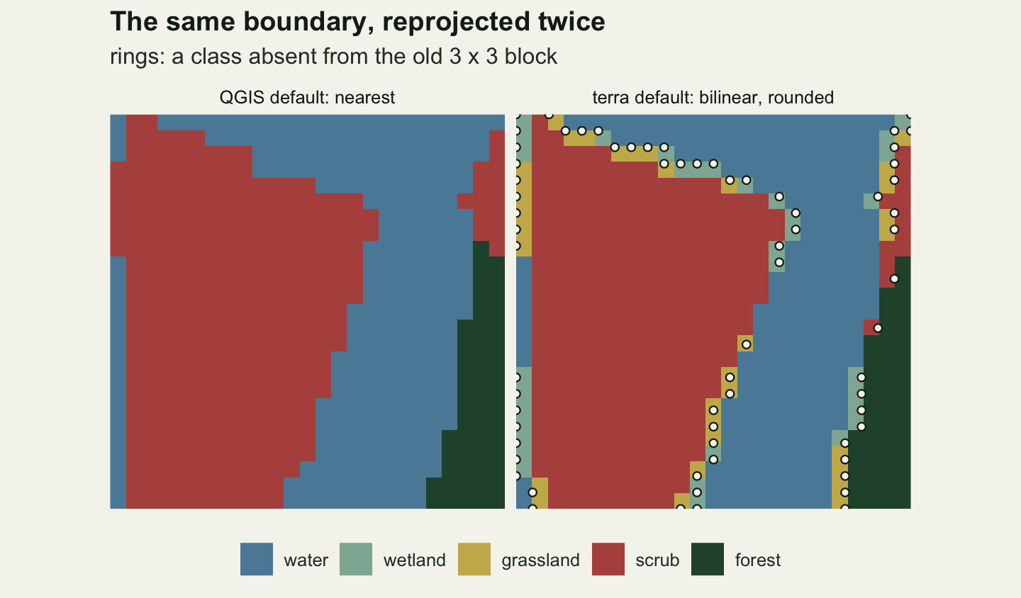
How much of a map this touches depends on how much of it lies on a boundary, because bilinear only makes a non-integer value where the four old cells around a point disagree. The chunk below repeats the check on five new maps built the same way, with fewer or more patches, and records for each the share of old cells next to a different class, which you can compute for your own map before reprojecting it.
n_patches <- c(20, 70, 250, 900, 3200); set.seed(20261014)
sweep <- data.frame(patches = n_patches, t(sapply(n_patches, function(n) {
  lc <- voronoi_cover(n); code_check(lc, project(lc, stereo)) })))
ratio_nonint <- range(sweep$non_int / sweep$edge)
ratio_inv    <- range(sweep$invented / sweep$edge)
The share of output cells with a non-integer value runs from 0.50 to 0.61 times the share of old cells on a boundary, and the share with an invented class from 0.15 to 0.17 times. On the most fragmented of the five maps, 80 per cent of the old cells are on a boundary, 49 per cent of the output is not a whole number and 12 per cent is an invented class. The more scattered single cells a classification has, the further towards that end it sits.
Telling terra that the codes are classes
The usual advice, as in Lovelace, Nowosad and Muenchow’s Geocomputation with R (2019; free online as a later edition at r.geocompx.org), is nearest neighbour for a categorical raster and bilinear for a continuous one. The catch is that terra can only follow it if the raster says which kind it is. There are two fixes on the R side and both are one line. Pass method = "near", or give the raster its category table before projecting, so that terra knows the codes are labels. With the table in place the default switches to nearest, and the output keeps the table.
cover_lab <- cover
levels(cover_lab) <- data.frame(id = 1:5, cover = classes)
t_lab <- project(cover_lab, stereo)
lab_is_factor <- is.factor(t_lab)
lab_same <- identical(as.vector(values(t_lab)), as.vector(values(t_near)))
stopifnot(lab_is_factor, lab_same)
The projected map with a category table is still a factor, and its cells are identical to those from method = "near". Setting the table is the better habit of the two, because it also travels with the map into plot(), freq() and anything else that reads categories.
A DEM: nearest keeps the values, bilinear keeps the shape
For an elevation model the question turns round. Averaging elevations is what you want; copying a cell that is up to half a cell away moves the surface sideways. The QGIS default and the terra default are compared below on the elevation model, with the two QGIS outputs read from their files.
q_dem_near <- rast("qgis-dem-near.tif"); q_dem_bil <- rast("qgis-dem-bilinear.tif")
t_dem_bil  <- project(dem, stereo); t_dem_near <- project(dem, stereo, method = "near")
dem_diff_near <- sum(values(q_dem_near)[, 1] != values(t_dem_near)[, 1], na.rm = TRUE)
dem_gap_bil   <- max(abs(values(q_dem_bil)[, 1] - values(t_dem_bil)[, 1]), na.rm = TRUE)
peak_in <- function(r, xy, half) {       # highest cell within a square around a point
  e <- ext(xy[1] - half, xy[1] + half, xy[2] - half, xy[2] + half)
  if (crs(r) != crs(dem)) e <- ext(project(e, utm, stereo))
  max(values(crop(r, e)), na.rm = TRUE)
}
dem_row <- function(r) {
  v <- values(r)[, 1]
  c(min = min(v, na.rm = TRUE), max = max(v, na.rm = TRUE), mean = mean(v, na.rm = TRUE),
    hill = peak_in(r, hill_xy, 300), knoll = peak_in(r, knoll_xy, 150))
}
dem_tab <- rbind(dem_row(dem), dem_row(q_dem_near), dem_row(t_dem_bil))
rownames(dem_tab) <- c("old DEM, UTM 34N", "QGIS default (nearest)", "terra default (bilinear)")
knitr::kable(dem_tab, digits = 2, col.names = c("min", "max", "mean", "hill top", "knoll top"),
caption = "Elevation in metres, before and after reprojection to Stereo70.")| min | max | mean | hill top | knoll top | |
|---|---|---|---|---|---|
| old DEM, UTM 34N | 419.05 | 614.53 | 475.42 | 614.53 | 481.54 |
| QGIS default (nearest) | 419.05 | 614.53 | 475.42 | 614.53 | 481.54 |
| terra default (bilinear) | 419.27 | 614.31 | 475.42 | 614.31 | 478.80 |
knoll_drop <- dem_tab[1, "knoll"] - dem_tab[3, "knoll"]
tab_gap <- max(abs(dem_row(t_dem_near) - dem_row(q_dem_near)),
               abs(dem_row(q_dem_bil) - dem_row(t_dem_bil)))
mean_move <- max(abs(dem_tab[2:3, "mean"] - dem_tab[1, "mean"]))
hill_drop  <- dem_tab[1, "hill"] - dem_tab[3, "hill"]
QGIS’s nearest output matches project(method = "near") in all but 7 cells, and its bilinear output matches the terra default to within 2.5 millimetres, and swapping the tool behind either row changes no entry of the table by more than 1.5 millimetres. Nearest neighbour returns exactly the old minimum and maximum, because it only copies. Bilinear lowers the knoll top by 2.73 metres, 9 per cent of its 30 metre height, and the hill top by 0.22 metres: a weighted mean of four cells cannot exceed the highest of them, and how much it loses depends on how sharply the surface bends at the top. The knoll is a cone, as sharp as a summit gets at this cell size; the hill is broad. Neither mean moves by more than 0.002 metres.
knoll_s <- project(matrix(knoll_xy, 1), utm, stereo)
prof_row <- rowFromY(t_dem_bil, knoll_s[2])
prof_x   <- xFromCol(t_dem_bil, seq_len(ncol(t_dem_bil)))
near_x   <- abs(prof_x - knoll_s[1]) <= 240
prof_xy  <- cbind(prof_x[near_x], yFromRow(t_dem_bil, prof_row))
fine_x   <- seq(min(prof_xy[, 1]), max(prof_xy[, 1]), length.out = 400)
fine_utm <- project(cbind(fine_x, prof_xy[1, 2]), stereo, utm)
d0 <- prof_xy[, 1] - knoll_s[1]
prof_df <- rbind(data.frame(d = d0, z = extract(q_dem_near, prof_xy)[, 1], what = "QGIS default: nearest"),
                 data.frame(d = d0, z = extract(t_dem_bil, prof_xy)[, 1], what = "terra default: bilinear"))
true_df <- data.frame(d = fine_x - knoll_s[1], z = surface(fine_utm[, 1], fine_utm[, 2]))
ggplot(prof_df, aes(d, z)) +
  geom_line(data = true_df, colour = "grey55", linewidth = 1.6, alpha = 0.6) +
  geom_step(data = prof_df[prof_df$what == "QGIS default: nearest", ],
            aes(x = d - 15), colour = te_forest, linewidth = 0.7) +
  geom_line(data = prof_df[prof_df$what == "terra default: bilinear", ],
            colour = te_rust, linewidth = 0.8) +
  geom_point(aes(colour = what), size = 1.8) +
  scale_colour_manual(values = c(te_forest, te_rust), name = NULL) +
  labs(x = "distance east of the knoll centre (m)", y = "elevation (m)",
       title = "Nearest copies cells, bilinear rounds the top off",
       subtitle = "grey: the surface without noise") +
  theme_datasheet() + theme(legend.position = "bottom")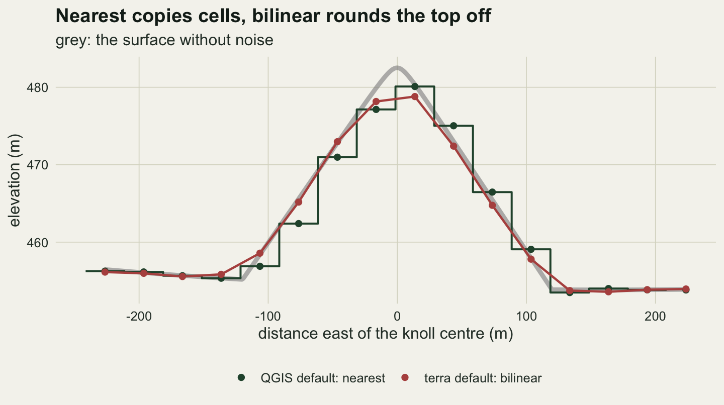
The price of nearest neighbour shows up in what is computed from the surface. The new grid is turned against the old one, so its rows run across the old rows at a small angle, and nearest neighbour settles the misfit in steps: along lines a fixed number of cells apart, the copied pattern jumps by one old row (or column). Slope is computed from differences between neighbouring cells, and across such a line the difference between two neighbouring new cells is taken between old cells that are also one row (or column) apart, so it picks up the slope in the other direction as well. The chunk measures the angle and computes slope with terrain() on the old DEM and on both outputs, against the slope of the noise-free surface at each cell centre.
ab <- project(rbind(c(652000, 5178000), c(653000, 5178000)), utm, stereo)
turn_deg <- atan2(ab[2, 2] - ab[1, 2], ab[2, 1] - ab[1, 1]) * 180 / pi
drift <- tan(abs(turn_deg) * pi / 180)   # how fast one grid's rows cross the other's
true_slope <- function(x, y, h = 0.01) {
  gx <- (surface(x + h, y) - surface(x - h, y)) / (2 * h)
  gy <- (surface(x, y + h) - surface(x, y - h)) / (2 * h)
  atan(sqrt(gx^2 + gy^2)) * 180 / pi
}
slope_err <- function(r) {
  s  <- values(terrain(r, "slope"))[, 1]
  xy <- xyFromCell(r, seq_len(ncell(r)))
  if (crs(r) != crs(dem)) xy <- project(xy, stereo, utm)
  s - true_slope(xy[, 1], xy[, 2])
}
err_old <- slope_err(dem); err_near <- slope_err(q_dem_near); err_bil <- slope_err(t_dem_bil)
slope_first <- project(terrain(dem, "slope"), stereo)   # slope in UTM, then reprojected
sf_xy <- project(xyFromCell(slope_first, seq_len(ncell(slope_first))), stereo, utm)
err_first <- values(slope_first)[, 1] - true_slope(sf_xy[, 1], sf_xy[, 2])
rmse <- function(e) sqrt(mean(e^2, na.rm = TRUE))
big_share <- function(e) mean(abs(e) > 2, na.rm = TRUE)
Here the Stereo70 grid is turned by 2.90 degrees against UTM zone 34 north. The rows of one grid drift across the rows of the other at the tangent of that angle, 5.07 per cent of a cell for every cell travelled, so there is a step every 20 cells or so in each direction.
The slope error, the computed slope minus the slope of the noise-free surface, has a root mean square of 0.47 degrees on the old DEM, where it is the half metre of noise talking. On QGIS’s nearest output it rises to 0.62 degrees, and 1.5 per cent of cells are more than 2 degrees out, against 0.2 per cent on the old DEM. On terra’s bilinear output it falls to 0.41 degrees, with 0.3 per cent over 2 degrees, because averaging four cells also averages away part of the noise. The seams are strongest where the ground is steep, on the flanks of the hill, and faint on the gentle ground to the east, because shifting the pattern by one cell changes an elevation difference by the local slope times the cell size. Computing slope first, on the old grid, and then reprojecting the slope raster with bilinear gives 0.41 degrees, with 0.3 per cent over 2 degrees.
seam_df <- rbind(
  data.frame(xyFromCell(q_dem_near, seq_len(ncell(q_dem_near))), err = err_near,
             panel = "QGIS default: nearest"),
  data.frame(xyFromCell(t_dem_bil, seq_len(ncell(t_dem_bil))), err = err_bil,
             panel = "terra default: bilinear"))
seam_df <- seam_df[!is.na(seam_df$err), ]
seam_plot <- ggplot(seam_df, aes(x, y, fill = pmax(-3, pmin(3, err)))) +
  geom_raster() + facet_wrap(~ panel) +
  scale_fill_gradient2(low = te_rust, mid = te_paper, high = te_forest, midpoint = 0,
                       limits = c(-3, 3), name = "slope error\n(degrees)") +
  coord_equal(expand = FALSE) +
  labs(x = NULL, y = NULL, title = "Nearest neighbour leaves seams in the slope map",
       subtitle = "computed slope minus true slope") +
  theme_datasheet() +
  theme(axis.text = element_blank(), panel.grid.major = element_blank())
seam_plot
Warning: Raster pixels are placed at uneven horizontal intervals and will be shifted
ℹ Consider using `geom_tile()` instead.
Raster pixels are placed at uneven horizontal intervals and will be shifted
ℹ Consider using `geom_tile()` instead.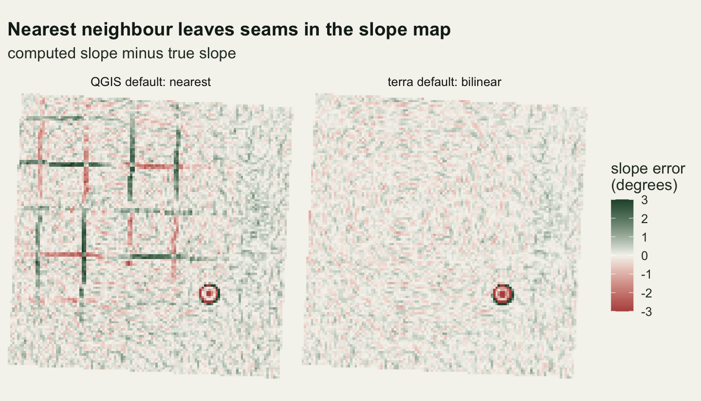
# a round trip: into Stereo70 and back onto the old grid, same method both ways
back_near <- project(t_dem_near, dem, method = "near"); back_bil <- project(t_dem_bil, dem)
d_near <- values(back_near)[, 1] - values(dem)[, 1]
d_bil  <- values(back_bil)[, 1] - values(dem)[, 1]
rt_exact <- mean(d_near == 0, na.rm = TRUE)
rt_knoll <- dem_tab[1, "knoll"] - peak_in(back_bil, knoll_xy, 150)
rt_bil_exact <- sum(d_bil == 0, na.rm = TRUE)
stopifnot(isTRUE(all.equal(rt_knoll, max(abs(d_bil), na.rm = TRUE))))   # the largest change is the knoll top
A round trip, into Stereo70 and back onto the original grid with the same method both ways, shows the two behaviours side by side. After nearest there and back, 97.4 per cent of the cells hold exactly their old value and the rest hold a neighbour’s, up to 5.62 metres away from their own. After bilinear, 3 cells out of 14399 hold exactly their old value, and the largest change anywhere is the knoll top, now 3.64 metres lower against 2.73 after one pass. Every reprojection of a surface costs something, so reproject once, from the original.
The output grid
Neither tool asks for a cell size. Both ask GDAL for a suggested output grid, and both got the same one.
res_auto <- res(t_default)[1]
corners  <- project(rbind(c(650000, 5182000), c(656000, 5176000)), utm, stereo)   # old diagonal
diag_res <- sqrt(sum(diff(corners)^2)) / sqrt(nrow(cover)^2 + ncol(cover)^2)
q_res30  <- rast("qgis-landcover-res30.tif")
t_res30  <- project(cover, stereo, res = 30, method = "near")
e_q <- as.vector(ext(q_res30)); e_t <- as.vector(ext(t_res30))
shift_y  <- e_q["ymax"] - e_t["ymax"]
diff_res30 <- sum(values(q_res30)[, 1] != values(t_res30)[, 1], na.rm = TRUE)
suggested <- as.vector(ext(t_default))
template <- rast(xmin = floor(suggested["xmin"] / 30) * 30, xmax = ceiling(suggested["xmax"] / 30) * 30,
                 ymin = floor(suggested["ymin"] / 30) * 30, ymax = ceiling(suggested["ymax"] / 30) * 30,
                 resolution = 30, crs = stereo)
q_tmpl <- rast("qgis-landcover-template.tif")
t_tmpl <- project(cover, template, method = "near")
tmpl_same <- isTRUE(all.equal(as.vector(ext(q_tmpl)), as.vector(ext(t_tmpl)))) &&
  all(dim(q_tmpl) == dim(t_tmpl))
diff_tmpl <- sum(values(q_tmpl)[, 1] != values(t_tmpl)[, 1], na.rm = TRUE)
tmpl_ext <- as.vector(ext(template))
stopifnot(tmpl_same)
The suggested cell is 30.0015 metres, not 30, because GDAL keeps the map’s diagonal as many cells long as before: the old diagonal, transformed, measures 30.0015 metres per old cell. Asking for 30 metres is Output file resolution in target georeferenced units in the Warp dialog (TARGET_RESOLUTION=30) and res = 30 in project(). Both then return 30 metre cells and the same number of rows and columns, but not the same grid: QGIS keeps the top edge of the suggested extent and terra the bottom edge, so the grids are offset by 0.316 metres north to south and 19 cells of the land-cover map differ.
The reliable way to get one grid is to write it down. In terra that is a template raster passed as the second argument of project(); here its edges are the suggested extent rounded outwards to whole multiples of 30 metres, 344400, 350730, 581820 and 588150 (west, east, south, north). In QGIS the same numbers go into Georeferenced extents of output file to be created (under Advanced Parameters) and the resolution into Output file resolution, which is what the qgis-landcover-template.tif command above did. The two grids are then identical, and the two nearest neighbour maps differ in 1 cell, the gdalwarp shortcut again. A template is also how to put a reprojected map exactly on top of another raster you already have: pass that raster.
What the screen shows is not the file
QGIS also resamples every time it draws a raster, because screen pixels never line up with raster cells. That setting is under Layer > Layer Properties > Symbology, in the Resampling frame, separately for zoomed in and zoomed out, and the default for new layers is under Settings > Options > Rendering, on the Raster tab, as the QGIS 3.40 user manual describes. It changes what you see and nothing in the file. According to the QGIS source (read, not measured here), a new layer gets nearest neighbour both ways: src/core/raster/qgsrasterlayer.cpp falls back to nearest neighbour in the 3.34, 3.40 and 3.44 branches and on master (checked 2026-09-25), and src/gui/raster/qgsresamplingutils.cpp shows an unset resampler as Nearest Neighbour in the Symbology tab. So a map that looks smooth in QGIS has had its display resampling changed, and a map that looks blocky may still have been reprojected with bilinear. Check the file, not the screen.
What to report
A methods section that says the land-cover map “was reprojected to Stereo70” leaves out the decision that changed it. Give the target CRS by its code, the datum transformation PROJ used, the resampling method and the output cell size, and say how the grid was fixed: “reprojected from UTM zone 34N (EPSG:32634) to Stereo70 (EPSG:3844) with nearest neighbour resampling onto a 30 m grid aligned to whole multiples of 30 m (terra project(), method near)”. For a categorical map at a similar cell size, nearest neighbour is the method that keeps every code real, and a reader who sees bilinear will know the class boundaries were smeared. For an elevation model, say which one you used and if slope or another derivative comes from a surface that was reprojected with nearest neighbour, compute it on the original grid instead and reproject the result. If the analysis compares class shares or patch counts before and after, say that the numbering of the classes played no part, which is true only with nearest neighbour.
Where the defaults are set
The QGIS files were made by QGIS 3.34.4 on Linux over GDAL 3.8.4 and PROJ 9.4.0; the R side of this page ran on terra 1.9.34 over GDAL 3.8.5 and PROJ 9.5.1. The terra rule quoted above sits at the top of the project() method for SpatRaster, in R/generics.R, and is the same in terra 1.7.65 and in the rspatial/terra repository on GitHub at version 1.9-51 (the commit of 2026-09-16); the defaults chunk checks it again on whichever version builds the page. resample() has the same rule in current terra, while 1.7.65 checks only whether the raster is a factor. The Warp page of the QGIS 3.40 user manual gives the same default as the qgis_process help. The -et shortcut and its default of an eighth of a cell are in the gdalwarp documentation, and the diagonal rule for the suggested cell size is coded in GDALSuggestedWarpOutput2(), in GDAL’s alg/gdaltransformer.cpp.
Honest limits
The measurements are on two synthetic rasters, one pair of coordinate systems and a turn of 2.9 degrees between them. A larger turn, as between a UTM zone and a national grid far from its central meridian, puts the nearest neighbour steps closer together. The transformation from UTM on WGS 84 to Stereo70 includes a datum shift, and PROJ has several candidate operations for Romania. The one used here, Pulkovo 1942(58) to WGS 84 (19), with a stated accuracy of 3 metres, is the default in both PROJ 9.4.0 and 9.5.1, and the two give coordinates equal to within a millionth of a metre (checked with sf and pyproj, outside this page); a different PROJ database could pick another operation and shift the whole grid, and the stopifnot() lines in the chunks then stop the page from building rather than compare mismatched grids. The land-cover patches are convex areas around random centres with random codes, so boundaries between distant codes are as common as between close ones; a map numbered so that neighbouring classes have neighbouring codes would invent fewer classes, and the count of invented cells depends on the numbering in a way no rule of thumb captures. The ratios in the sweep come from one map at each fragmentation level. The slope comparison uses a surface with half a metre of noise and one sharp feature; on a very smooth surface the nearest neighbour seams are smaller, and on a rougher one bilinear removes more of the roughness along with the noise, which is a change to the data in its own right. Only nearest and bilinear were compared; cubic and the aggregating methods (average, mode) were not, and mode or average are the usual choices when the new cells are much larger than the old. Reprojection to longitude and latitude, where cells stop being square on the ground, was not measured. QGIS Export > Save As with a different CRS reprojects through QGIS’s own code rather than gdalwarp and offers no resampling choice (read from the QGIS 3.34 source, not measured here).
References
Lovelace R, Nowosad J, Muenchow J 2019 Geocomputation with R. Chapman and Hall/CRC (ISBN 9781138304512; 10.1201/9780203730058)