library(sf)
library(terra)
library(ggplot2)
terraOptions(progress = 0)

te_paper  <- "#f5f4ee"; te_ink    <- "#16241d"; te_body   <- "#2c3a31"
te_forest <- "#275139"; te_rust   <- "#b5534e"; te_gold   <- "#c9b458"
te_line   <- "#dad9ca"

theme_datasheet <- function() {
  theme_minimal(base_size = 12) +
    theme(plot.background  = element_rect(fill = te_paper, colour = NA),
          panel.background = element_rect(fill = te_paper, colour = NA),
          panel.grid.major = element_line(colour = te_line, linewidth = 0.3),
          panel.grid.minor = element_blank(),
          text             = element_text(colour = te_body),
          plot.title       = element_text(colour = te_ink, face = "bold"),
          plot.subtitle    = element_text(colour = te_body),
          axis.text        = element_text(colour = te_body))
}

soft      <- sf_extSoftVersion()
sf_ver    <- as.character(packageVersion("sf")); terra_ver <- as.character(packageVersion("terra"))
geos_r <- unname(soft["GEOS"]); gdal_r <- unname(soft["GDAL"]); proj_r <- unname(soft["PROJ"])Running QGIS from the command line
R
QGIS
GIS
spatial
ecology tutorial
Scripting QGIS with qgis_process, and measuring where its algorithms match sf and terra exactly and where a different default moves an ecological number.
Corrected 27 September 2026: the spatial join section said that st_join offers the one to many and first match rules but not the largest overlap rule; it is the other way round, since st_join(..., largest = TRUE) gives the largest overlap and there is no first match option.
Six habitat patches and twelve point count stations sit in a block of survey area two kilometres by one and a half, with a canopy height raster on a fifty metre grid over the top. Three ordinary jobs follow. Put a hundred metre foraging radius around each station and record which habitats it reaches. Merge the patches into forest and wetland. Take mean canopy height inside each patch. All three are in the QGIS Processing toolbox, and all three are in sf and terra.
The other QGIS post on this site, From QGIS to R: a spatial join with GeoPackage, walks the first of those through the graphical interface and hands the result to sf. It says plainly that the join is one line of sf, and that this is not a case where QGIS does something R cannot. The parts of QGIS that have no R equivalent are elsewhere: the print composer, on screen digitising, the georeferencer, the interactive styling of a layer you have never seen before. Steiniger and Hunter’s survey of the open source GIS field is a reminder of how much of a desktop GIS is not an algorithm at all. None of that is measured here, and this post makes no claim about it. The question it can answer is narrower. For the operations that are algorithms on both sides, does the toolbox return the same numbers as sf and terra, and what does it do differently when you accept its defaults? Part of the usual objection to the toolbox is that it is not reproducible, because clicking is not a script. That part is wrong, and has been for years. QGIS ships qgis_process, a command line runner that reaches every algorithm in the toolbox, takes parameters as flags and prints machine readable results. Sandve and colleagues make the general case for recording every step as an executable command rather than as a memory of what was clicked; qgis_process is what makes that possible for the QGIS half of a pipeline.
One constraint shapes the whole page: no chunk here calls QGIS, because the page has to build on a machine that does not have it. So the QGIS side is a transcript. Every QGIS command ran once against QGIS 3.34.4-Prizren in a Linux container, each command appears below in a plain fenced block that Quarto does not execute, and its output is copied into a chunk as a literal. The sf and terra numbers beside them are computed live, on whatever machine builds the page, which is not that container. Every gap quoted below is therefore a difference between two machines as well as between two toolchains, unless the two library stacks happen to match; the next section checks whether they do. Versions matter more here than usual anyway, because algorithm identifiers and parameter names move between major releases, and yours may differ.
The R side of this page ran on sf 1.1.1 and terra 1.9.34, over GEOS 3.13.0, GDAL 3.8.5 and PROJ 9.5.1. Those three libraries do the geometry, the file reading and the reprojection, in R and in QGIS alike, which is why the comparison below has any chance of coming out even. Bivand traces how the R spatial packages came to sit on that stack; sf is Pebesma’s interface to it and terra is Hijmans’s.
The layers, and the files the commands need
Everything is synthetic, in metres, on UTM zone 34 north, so the true areas are known and nothing depends on a download. The patches are rectangles at deliberately untidy coordinates, so that almost none of their edges land on a raster cell boundary. That is what makes the last section possible.
utm <- "EPSG:32634"; x_org <- 400000; y_org <- 5050000; scratch <- tempdir()
rect_of <- function(xa, xb, ya, yb)
  st_polygon(list(cbind(x_org + c(xa, xb, xb, xa, xa),
                        y_org + c(ya, ya, yb, yb, ya))))
patches <- st_sf(
  patch_id = sprintf("P%02d", 1:6),
  habitat  = c("forest", "forest", "wetland", "wetland", "forest", "wetland"),
  geometry = st_sfc(rect_of(117, 497, 106, 403), rect_of(497, 803, 106, 403),
                    rect_of(906, 1259, 143, 397), rect_of(1259, 1512, 143, 397),
                    rect_of(213, 511, 604, 811), rect_of(907, 1311, 641, 952),
                    crs = utm))
n_site  <- 12; set.seed(20260811)
site_xy <- cbind(runif(n_site, 60, 1640), runif(n_site, 60, 1000))
sites   <- st_sf(site_id = sprintf("S%02d", seq_len(n_site)),
                 geometry = st_sfc(lapply(seq_len(n_site), function(i)
                   st_point(c(x_org, y_org) + site_xy[i, ])), crs = utm))
one_pt  <- st_sf(id = 1L, geometry = st_sfc(st_point(c(x_org + 800, y_org + 500)), crs = utm))
canopy  <- rast(xmin = x_org, xmax = x_org + 2000, ymin = y_org,
                ymax = y_org + 1500, resolution = 50, crs = utm)
cell_xy <- xyFromCell(canopy, seq_len(ncell(canopy))); set.seed(4677)
values(canopy) <- round(8 + 10 * (cell_xy[, 2] - y_org) / 1500 +
                          rnorm(ncell(canopy), 0, 1.2), 3)
gpkg <- function(x, nm) st_write(x, file.path(scratch, nm), delete_dsn = TRUE, quiet = TRUE)
gpkg(patches, "patches.gpkg"); gpkg(sites, "sites.gpkg"); gpkg(one_pt, "one_point.gpkg")
writeRaster(canopy, file.path(scratch, "canopy.tif"), overwrite = TRUE, datatype = "FLT8S")
cell_m <- res(canopy)[1]; patch_area <- as.numeric(st_area(patches))
6 patches covering 54.5 hectares, 12 stations, one lone point for the buffer calls, and a canopy raster of 1200 cells at 50 metres. That chunk writes three GeoPackages and a GeoTIFF into a scratch directory. The small feature layer of the last section is a fifth file, written there rather than here; every command below assumes you have changed into that directory.
The toolbox has a command line
Three subcommands cover almost everything: list prints every algorithm the installation can see, help prints the parameters of one, and run executes it. Nothing needs a display, so QT_QPA_PLATFORM=offscreen is enough to run it on a headless server.
export QT_QPA_PLATFORM=offscreen
qgis_process list | grep -E "(native|gdal):buffer(vectors)?\s"
gdal:buffervectors Buffer vectors
native:buffer BufferThe prefix on an identifier is not decoration; it names the engine that does the work. native: algorithms are compiled into QGIS and call GEOS directly, gdal: algorithms build a GDAL command line and shell out to it, and qgis: algorithms are the older Python implementations. Two algorithms with similar names and different prefixes are two different programs, and the next section has them returning two different circles from one request. The help page is the only place the defaults are written down.
qgis_process help native:buffer | grep -A1 -E "^(DISTANCE|SEGMENTS):"DISTANCE: Distance
Default value: 10
--
SEGMENTS: Segments
Default value: 5Running an algorithm means putting the parameters after a bare double hyphen in KEY=value form, with file paths for inputs and outputs, so the call composes with anything else that reads and writes GeoPackages. Adding --json returns a document rather than a paragraph. That document is long for one dissolve, so the two parts worth reading are pulled out of the saved file with grep and tail: the header names the libraries this QGIS is using, and the tail carries the results.
qgis_process run native:dissolve --json -- INPUT=patches.gpkg FIELD=habitat OUTPUT=dissolved.gpkg > dissolve.json
grep -E '"(gdal|geos|proj)_version"' dissolve.json
tail -4 dissolve.json
"gdal_version": "3.8.4",
"geos_version": "3.12.1-CAPI-1.18.1",
"proj_version": "Rel. 9.4.0, March 1st, 2024",
"results": {
"OUTPUT": "dissolved.gpkg"
}
}gdal_q <- "3.8.4"; geos_q <- "3.12.1"; proj_q <- "9.4.0" # from the header above
stack_same <- identical(c(gdal_r, geos_r, proj_r), c(gdal_q, geos_q, proj_q))
stack_word <- if (stack_same) "matches the container exactly" else "does not match it"
# six wall clock times of one QGIS command line call, and six per cycle means of twenty
# read, buffer and write cycles in R, both transcribed from the same container: seconds
qgis_wall <- c(1.34, 1.30, 1.33, 1.31, 1.39, 1.32)
r_wall <- c(0.0180, 0.0156, 0.0159, 0.0152, 0.0172, 0.0163)
qgis_mean_s <- mean(qgis_wall); qgis_sd_s <- sd(qgis_wall); r_mean_s <- mean(r_wall)
call_ratio <- qgis_mean_s / r_mean_sCompare those version strings with what the setup chunk printed from sf_extSoftVersion(). The stack this page was built on does not match it. Where they differ, a small residual in the tables below is a difference between two builds rather than a property of either tool, and that is the first thing worth checking when two answers disagree. The cost of the command line is startup, and both halves of that measurement are transcripts from the container, so the ratio below is one machine divided by itself: six calls to a trivial buffer against six blocks of twenty read, buffer and write cycles in R. A qgis_process call took 1.33 seconds of wall clock, with a standard deviation over the six repeats of 0.03, essentially all of it spent starting a QGIS application. The same work in R took 0.016 seconds, a factor of about 81. That cost is paid once per call, so it is nothing on one dissolve of a national dataset and ruinous inside a loop over a thousand features. If a QGIS step has to run per feature, hand it the whole layer in one call.
The buffer default is where the two toolchains part company
A foraging radius is a buffer, and a buffer is a circle approximated by a polygon. Its vertices sit on the true circle, so the polygon is inscribed and its area is short by an amount with a closed form: for a regular polygon of n vertices the ratio to the circle is (n / (2 * pi)) * sin(2 * pi / n). The companion post Choosing a projection for area and distance derives that identity and checks it against st_buffer, so it is taken as known here. What matters now is that both toolchains take the same argument, count it the same way as segments per quarter circle, and set it to different values.
qgis_process run native:buffer -- INPUT=one_point.gpkg DISTANCE=1000 OUTPUT=buf_default.gpkg
qgis_process run native:buffer -- INPUT=one_point.gpkg DISTANCE=1000 SEGMENTS=30 OUTPUT=buf_30.gpkg
qgis_process run gdal:buffervectors -- INPUT=one_point.gpkg GEOMETRY=geom DISTANCE=1000 OUTPUT=buf_gdal.gpkg
ngon_ratio <- function(n) (n / (2 * pi)) * sin(2 * pi / n); buf_r <- 1000
seg_sf <- eval(formals(sf::st_buffer)$nQuadSegs) # what sf uses by default
seg_qg <- 5 # what native:buffer uses by default
# areas and vertex counts read back from the three output GeoPackages above
qgis_area <- c(3090169.943749577, 3140157.374576814, 3140157.374576814)
qgis_verts <- c(20, 120, 120)
buf_tab <- data.frame(
call = c("native:buffer default", "native:buffer SEGMENTS=30",
"gdal:buffervectors default"),
vertices = qgis_verts, qgis_m2 = qgis_area,
sf_m2 = vapply(c(seg_qg, seg_sf, seg_sf), function(q)
as.numeric(st_area(st_buffer(one_pt, buf_r, nQuadSegs = q))), 0),
closed_form = pi * buf_r^2 * ngon_ratio(qgis_verts))
buf_tab$deficit_pct <- 100 * (1 - buf_tab$qgis_m2 / (pi * buf_r^2))
knitr::kable(buf_tab, row.names = FALSE, digits = c(0, 0, 4, 4, 4, 4),
caption = "One point, one distance, three buffer calls.")| call | vertices | qgis_m2 | sf_m2 | closed_form | deficit_pct |
|---|---|---|---|---|---|
| native:buffer default | 20 | 3090170 | 3090170 | 3090170 | 1.6368 |
| native:buffer SEGMENTS=30 | 120 | 3140157 | 3140157 | 3140157 | 0.0457 |
| gdal:buffervectors default | 120 | 3140157 | 3140157 | 3140157 | 0.0457 |
gap_qs   <- max(abs(buf_tab$qgis_m2 - buf_tab$sf_m2))
gap_cf   <- max(abs(buf_tab$qgis_m2 - buf_tab$closed_form))
def_qg   <- buf_tab$deficit_pct[1]; def_sf <- buf_tab$deficit_pct[2]
forage_r <- 100; forage_ha <- pi * forage_r^2 / 1e4; ha_lost <- (def_qg - def_sf) / 100 * forage_ha
The three QGIS answers land on the three sf answers, and on the closed form for the same polygon, to within floating-point rounding on an area of three square kilometres. There is no numerical disagreement in that table. The disagreement is entirely about which row you get when you type nothing. At the QGIS default of 5 segments per quarter circle the buffer is short by 1.64 per cent. At the sf default of 30 it is short by 0.046 per cent. On a 100 metre foraging circle that is 0.0500 hectares out of 3.14. Because it is the same fraction on every circle it is a bias and not a scatter: every buffer derived area comes out 1.59 per cent smaller than the same buffer built in R.
seg_grid <- data.frame(segments = 1:40)
seg_grid$deficit_pct <- 100 * (1 - ngon_ratio(4 * seg_grid$segments))
mark <- data.frame(segments = c(seg_qg, seg_sf), deficit_pct = c(def_qg, def_sf),
                   lab = c("QGIS native:buffer default", "sf and GDAL default"))
ggplot(seg_grid, aes(segments, deficit_pct)) +
  geom_line(colour = te_body, linewidth = 0.7) +
  geom_point(data = mark, aes(colour = lab), size = 3.4) +
  geom_text(data = mark, aes(label = lab, colour = lab), hjust = -0.09,
            size = 3.3, show.legend = FALSE) +
  scale_x_log10(breaks = c(1, 2, 5, 10, 20, 40), limits = c(1, 130)) +
  scale_y_log10(breaks = c(0.03, 0.1, 0.3, 1, 3, 10, 30)) +
  scale_colour_manual(values = c("QGIS native:buffer default" = te_rust,
                                 "sf and GDAL default" = te_forest), name = NULL) +
  labs(x = "segments per quarter circle (log scale)",
       y = "area deficit (per cent, log scale)",
       title = "The buffer default costs a fixed fraction of every circle",
       subtitle = "inscribed polygon against the true circle, closed form") +
  theme_datasheet() + theme(legend.position = "none")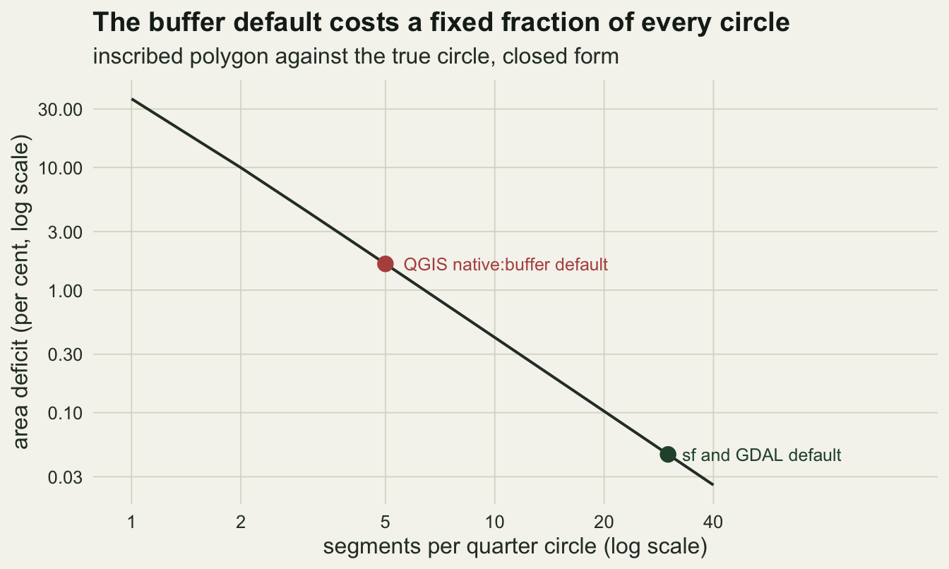
The third row of the table is the one to stare at. gdal:buffervectors is a QGIS algorithm run through the same command line, and it returns the sf answer rather than the QGIS one, because it is not QGIS geometry code: it builds an ogr2ogr call, and GDAL’s own buffer uses thirty segments per quadrant. One toolbox, one GEOS underneath, two defaults, and the prefix is the only thing that says which you are about to get. That algorithm also shows the least pleasant property of the gdal: provider: its GEOMETRY parameter defaults to a column named geometry, while the GeoPackage sf writes calls its geometry column geom, so leaving the default alone produces this on standard error:
ERROR:  ERROR 1: In ExecuteSQL(): sqlite3_prepare_v2(SELECT ST_Buffer(geometry, 1000.0) AS geometry,* FROM "one_point"):
  no such column: geometry
ERROR:  Process returned error code 1
after which qgis_process exits with status zero and leaves a sixty four kilobyte GeoPackage on disk that no reader can open. A pipeline that checks the exit code, or checks that the output file exists, walks straight past that; checking that the output layer has the number of features you expected is what catches it. A missing input file or a misspelled identifier do return status one, so the failure is specific to the shelled out provider.
Dissolve and join give the same geometry and different bookkeeping
Merging the six patches into forest and wetland is native:dissolve on one side and aggregate over a union on the other. Both end at the same GEOS call, and the dissolve was already run above.
# areas read back from dissolved.gpkg, written by the native:dissolve call above
qgis_diss <- c(forest = 265428, wetland = 279568)
diss_sf <- aggregate(patches["habitat"], by = list(habitat = patches$habitat),
                     FUN = function(z) z[1], do_union = TRUE)
diss_sf  <- diss_sf[order(diss_sf$habitat), ]
sf_diss  <- setNames(as.numeric(st_area(diss_sf)), diss_sf$habitat)
diss_gap <- max(abs(qgis_diss - sf_diss[names(qgis_diss)]))
n_part   <- vapply(st_geometry(diss_sf), length, 0L)
The two areas differ by 0 square metres, and both classes come back as 2 part multipolygons, because two of the three forest rectangles share an edge and merge while the third does not. The geometries are not merely equal in area: run the check below in a container that has both installed and the well known binary of each dissolved feature is identical byte for byte, once the sf result is promoted to MULTIPOLYGON as the GeoPackage format does to the QGIS output.
qgis_out <- st_read("dissolved.gpkg", quiet = TRUE)
identical(st_as_binary(st_cast(st_geometry(diss_sf), "MULTIPOLYGON")),
          st_as_binary(st_geometry(qgis_out)))
The difference is in the attributes, and it is silent. QGIS keeps the whole attribute row of the first feature in each group, so the dissolved forest polygon still carries patch_id of P01, a label that now describes a third of the geometry attached to it. Nothing in the output marks it as stale. The join is where that bookkeeping starts to matter, because a hundred metre circle can reach two patches or none. Without --json each call answers with a paragraph of echoed inputs and a progress line, and only the last lines of that are the results, tab separated. Both calls below are tailed to exactly those lines, so the block underneath them is the whole of what they print: one result key from the buffer, two from the join.
qgis_process run native:buffer -- INPUT=sites.gpkg DISTANCE=100 SEGMENTS=30 OUTPUT=forage.gpkg | tail -1
qgis_process run native:joinattributesbylocation -- INPUT=forage.gpkg JOIN=patches.gpkg PREDICATE=0 METHOD=0 JOIN_FIELDS=habitat OUTPUT=joined.gpkg | tail -2
OUTPUT: forage.gpkg
JOINED_COUNT: 11
OUTPUT: joined.gpkgforage <- st_buffer(sites, forage_r)
hit <- lengths(st_intersects(forage, patches))
join_many <- st_join(forage, patches["habitat"], join = st_intersects)
join_inner <- st_join(forage, patches["habitat"], join = st_intersects, left = FALSE)
# row counts and the sorted station and habitat pairs, read back from the QGIS outputs
qgis_rows <- c(one_to_many = 15, one_to_one = 12, discard_nonmatching = 11)
qgis_joined_count <- 11
qgis_pairs <- c("S01 forest", "S02 NA", "S03 wetland", "S03 wetland", "S04 wetland",
"S05 forest", "S05 forest", "S06 wetland", "S07 forest", "S07 wetland",
"S08 NA", "S09 NA", "S10 wetland", "S11 wetland", "S12 NA")
sf_rows <- c(one_to_many = nrow(join_many), one_to_one = nrow(forage),
discard_nonmatching = nrow(join_inner))
sf_pairs <- sort(paste(join_many$site_id,
ifelse(is.na(join_many$habitat), "NA", join_many$habitat)))
row_gap <- max(abs(qgis_rows - sf_rows)); pair_same <- identical(sf_pairs, sort(qgis_pairs))
pair_agree <- sum(sf_pairs == sort(qgis_pairs)); n_na <- sum(is.na(join_many$habitat))
n_zero <- sum(hit == 0); n_one <- sum(hit == 1); n_two <- sum(hit > 1)4 circles reach no patch, 5 reach exactly one and 3 reach two, so a one to many join of 12 features has to produce 15 rows. QGIS produced the same, and all three row counts matched, with a largest discrepancy of 0. Sorting the station and habitat pairs from both outputs gives vectors that agree on 15 of 15 entries, and identical() on the two sorted vectors is TRUE, so this is agreement on content and not a coincidence of totals. Those fifteen pairs are the one place where a transcribed QGIS result carries content rather than a count.
loc_g <- function(x) st_sfc(st_geometry(x) - c(x_org, y_org))
reach <- c("no patch", "one patch", "two patches")[hit + 1]
p_loc <- st_sf(habitat = patches$habitat, geometry = loc_g(patches))
ggplot() +
  geom_sf(data = p_loc, aes(fill = habitat), colour = NA, alpha = 0.5) +
  geom_sf(data = st_sf(reach = reach, geometry = loc_g(forage)),
          aes(colour = reach, linetype = reach), fill = NA, linewidth = 0.8) +
  scale_fill_manual(values = c(forest = te_forest, wetland = te_gold), name = NULL) +
  scale_colour_manual(values = c("no patch" = te_body, "one patch" = te_forest,
                                 "two patches" = te_rust), name = NULL) +
  scale_linetype_manual(values = c("no patch" = "dotted", "one patch" = "solid",
                                   "two patches" = "solid"), name = NULL) +
  labs(x = "metres east", y = "metres north",
       title = sprintf("%d circles, %d join rows", n_site, sf_rows[["one_to_many"]]),
       subtitle = "hundred metre foraging radius over six habitat patches") +
  theme_datasheet() + theme(legend.position = "bottom")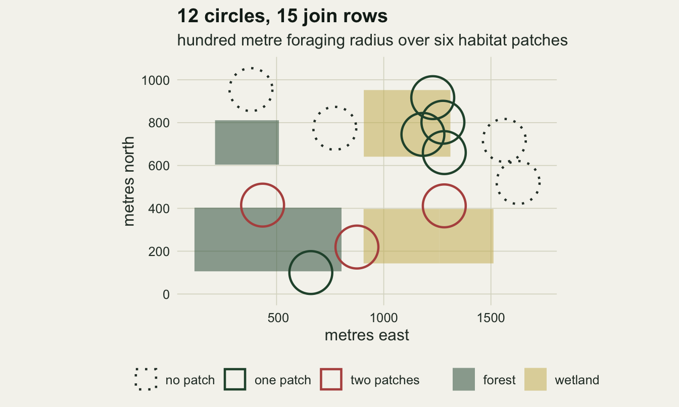
Two things in that output still need reading carefully. JOINED_COUNT came back as 11, which is neither the number of output rows nor the number of input features: it counts rows that carry a joined attribute, which is 15 minus the 4 unmatched circles. And the rows arrive in a different order, because QGIS emits matched features in the order its spatial index visits them and appends the unmatched at the end, while st_join preserves the order of the input layer. Anything downstream that uses row position rather than an identifier is a bug waiting for a large enough layer. DISCARD_NONMATCHING=1 is left = FALSE, and it removes the 4 stations that reached no habitat: those stations are data, they are the ones sitting in the matrix between patches, and dropping them silently turns a question about habitat use into a question about habitat use given that there was habitat. The METHOD parameter is the last flag to set deliberately. Method zero is one to many, method one takes the first matching feature, and method two takes the feature with the largest overlap. st_join has the first and the third, the third through largest = TRUE; it has no first match option, so that rule has to be written out. The chunk below writes both one to one rules out from st_intersects(), so that each step is visible.
# habitat per station under the two one-to-one methods, read back from QGIS output,
# one letter per station in station order: f forest, w wetland, n no match
lut <- c(f = "forest", w = "wetland", n = NA)
qgis_first  <- unname(lut[strsplit("fnwwfwfnnwwn", "")[[1]]])
qgis_larger <- unname(lut[strsplit("fnwwfwwnnwwn", "")[[1]]])
touch <- st_intersects(forage, patches)
sf_first <- vapply(touch, function(k)
  if (!length(k)) NA_character_ else patches$habitat[k[1]], character(1))
sf_larger <- vapply(seq_along(touch), function(i) {
  k <- touch[[i]]; if (!length(k)) return(NA_character_)
  ov <- as.numeric(st_area(st_intersection(st_geometry(forage)[i],
                                           st_geometry(patches)[k])))
  patches$habitat[k[which.max(ov)]]
}, character(1))
match_n  <- function(a, b) sum(a == b | (is.na(a) & is.na(b)), na.rm = TRUE)
n_first  <- match_n(sf_first, qgis_first); n_larger <- match_n(sf_larger, qgis_larger)
n_switch <- sum(!is.na(qgis_first) & qgis_first != qgis_larger)
Both reproduce exactly: the first matching rule agrees with sf taking the first index on 12 of 12 stations, and the largest overlap rule, computed from the intersection areas, agrees with the QGIS one on all 12 as well. The two rules disagree with each other on 1 of the 3 stations that reach two patches. That station is labelled forest by one rule and wetland by the other, on a circle whose forest share is the smaller of the two. The first matching rule picks by feature order in the join layer, which is a property of how the file was written.
Zonal statistics switch rule at two captured cell centres
Mean canopy height per patch is native:zonalstatisticsfb in QGIS and terra::extract in R. Both have to decide which pixels belong to a polygon whose edges do not follow the grid, and the sibling post Rasterising a vector layer measures what that decision is worth. Here the question is only whether the two tools make the same one.
qgis_process run native:zonalstatisticsfb -- INPUT=patches.gpkg INPUT_RASTER=canopy.tif COLUMN_PREFIX=z_ STATISTICS=0,1,2 OUTPUT=zonal.gpkg# count and mean columns read back from zonal.gpkg
qgis_zn <- c(48, 36, 35, 25, 24, 48)
qgis_zm <- c(9.678541666667, 9.771777777778, 9.908657142857,
9.915840000000, 12.827666666667, 12.996291666667)
patch_v <- vect(patches)
centre_n <- extract(canopy, patch_v, fun = function(z, ...) sum(!is.na(z)))[, 2]
centre_m <- extract(canopy, patch_v, fun = mean, na.rm = TRUE)[, 2]
zn_gap <- max(abs(qgis_zn - centre_n)); zm_gap <- max(abs(qgis_zm - centre_m))On these six patches the two agree exactly: the pixel counts differ by 0 and the means agree to the twelve decimal places the QGIS output was copied with. Both apply the cell centre rule, in which a pixel belongs whole to the patch whose polygon contains the pixel’s centre, with no weight for how much of it actually lies inside. The smallest of these patches still captures 24 cell centres, which turns out to be the reason. That agreement stops holding for small features. Ponds, sinkholes, single trees and quadrats are routinely smaller than a satellite or elevation model pixel. The layer below holds two sets of rectangles. The sweep is eight squares from half a cell across to eight cells across, all sharing one centre point and so one offset from the grid. The probes are five rectangles placed on purpose: two squares centred on a cell centre, one square centred on a cell corner instead, and two thin rectangles, one standing tall enough to catch a cell centre in each of two rows and one lying flat between two rows.
box_spec <- data.frame(
  feature = c(sprintf("W%d", 1:8), "A", "B", "C", "D", "E"),
  cx = c(rep(238, 8), 225, 225, 250, 225, 250),
  cy = c(rep(217, 8), 225, 225, 250, 250, 250),
  w  = c(25, 40, 60, 75, 100, 150, 250, 400, 95, 80, 60, 45, 300),
  h  = c(25, 40, 60, 75, 100, 150, 250, 400, 95, 80, 60, 95, 45),
  layer = rep(c("sweep", "probe"), c(8, 5)))
boxes <- st_sf(box_spec, geometry = st_sfc(lapply(seq_len(nrow(box_spec)), function(i)
  rect_of(box_spec$cx[i] - box_spec$w[i] / 2, box_spec$cx[i] + box_spec$w[i] / 2,
          box_spec$cy[i] - box_spec$h[i] / 2, box_spec$cy[i] + box_spec$h[i] / 2)),
  crs = utm))
gpkg(boxes, "boxes.gpkg")
qgis_process run native:zonalstatisticsfb -- INPUT=boxes.gpkg INPUT_RASTER=canopy.tif COLUMN_PREFIX=z_ STATISTICS=0,2 OUTPUT=boxes_zonal.gpkgThe two candidate rules have to be written out to compare against. The cell centre rule is computed from the cell centres themselves rather than from terra::extract(fun = mean), because that function falls back to touched cells when a polygon captures no centre at all, which would quietly invent a value exactly where the rule has none. The area weighted rule is terra::extract(exact = TRUE), which returns the fraction of each cell that the polygon covers.
# count and mean columns read back from boxes_zonal.gpkg
qgis_bn <- c(0.25, 0.64, 1.44, 2, 4, 9, 25, 64, 3.61, 2.56, 4, 2, 5.4)
qgis_bm <- c(9.559500000000, 9.595680000000, 9.637430000000, 9.523500000000,
             9.546000000000, 9.405444444444, 9.512320000000, 9.301359375000,
             9.518119113573, 9.554437500000, 9.426750000000, 9.457000000000,
             9.549166666667)
cell_val <- values(canopy)[, 1]; frac <- extract(canopy, vect(boxes), exact = TRUE)
cell_pts <- st_as_sf(as.data.frame(cell_xy), coords = c("x", "y"), crs = utm)
caught   <- st_intersects(boxes, cell_pts)
box_tab  <- data.frame(
  feature = boxes$feature, layer = boxes$layer,
  wide_cells = boxes$w / cell_m, tall_cells = boxes$h / cell_m,
  area_cells = as.numeric(st_area(boxes)) / cell_m^2, centres = lengths(caught),
  qgis_count = qgis_bn, qgis_mean = qgis_bm,
  centre_mean = vapply(caught, function(k)
    if (!length(k)) NA_real_ else mean(cell_val[k]), 0),
  area_weighted_mean = as.numeric(tapply(seq_len(nrow(frac)), frac$ID, function(i)
    sum(frac[i, 2] * frac$fraction[i]) / sum(frac$fraction[i]))))
tol_m <- 1e-6      # terra's coverage fractions are themselves this approximate
as_c  <- abs(box_tab$qgis_count - box_tab$centres) < tol_m & !is.na(box_tab$centre_mean) &
  abs(box_tab$qgis_mean - box_tab$centre_mean) < tol_m
as_a  <- abs(box_tab$qgis_count - box_tab$area_cells) < tol_m &
  abs(box_tab$qgis_mean - box_tab$area_weighted_mean) < tol_m
box_tab$rule_used <- ifelse(as_c & !as_a, "cell centre",
                            ifelse(as_a & !as_c, "area weighted", "neither"))
knitr::kable(box_tab, row.names = FALSE, digits = c(0, 0, 2, 2, 2, 0, 2, 4, 4, 4, 0),
caption = "One raster, one command: eight squares on one grid offset, then five probes.")| feature | layer | wide_cells | tall_cells | area_cells | centres | qgis_count | qgis_mean | centre_mean | area_weighted_mean | rule_used |
|---|---|---|---|---|---|---|---|---|---|---|
| W1 | sweep | 0.5 | 0.5 | 0.25 | 0 | 0.25 | 9.5595 | NA | 9.5595 | area weighted |
| W2 | sweep | 0.8 | 0.8 | 0.64 | 1 | 0.64 | 9.5957 | 9.5610 | 9.5957 | area weighted |
| W3 | sweep | 1.2 | 1.2 | 1.44 | 1 | 1.44 | 9.6374 | 9.5610 | 9.6374 | area weighted |
| W4 | sweep | 1.5 | 1.5 | 2.25 | 2 | 2.00 | 9.5235 | 9.5235 | 9.6259 | cell centre |
| W5 | sweep | 2.0 | 2.0 | 4.00 | 4 | 4.00 | 9.5460 | 9.5460 | 9.5210 | cell centre |
| W6 | sweep | 3.0 | 3.0 | 9.00 | 9 | 9.00 | 9.4054 | 9.4054 | 9.4998 | cell centre |
| W7 | sweep | 5.0 | 5.0 | 25.00 | 25 | 25.00 | 9.5123 | 9.5123 | 9.4739 | cell centre |
| W8 | sweep | 8.0 | 8.0 | 64.00 | 64 | 64.00 | 9.3014 | 9.3014 | 9.4740 | cell centre |
| A | probe | 1.9 | 1.9 | 3.61 | 1 | 3.61 | 9.5181 | 9.5610 | 9.5181 | area weighted |
| B | probe | 1.6 | 1.6 | 2.56 | 1 | 2.56 | 9.5544 | 9.5610 | 9.5544 | area weighted |
| C | probe | 1.2 | 1.2 | 1.44 | 4 | 4.00 | 9.4268 | 9.4268 | 9.4268 | cell centre |
| D | probe | 0.9 | 1.9 | 1.71 | 2 | 2.00 | 9.4570 | 9.4570 | 9.4570 | cell centre |
| E | probe | 6.0 | 0.9 | 5.40 | 0 | 5.40 | 9.5492 | NA | 9.5492 | area weighted |
n_feat <- nrow(box_tab); n_none <- sum(box_tab$rule_used == "neither")
n_area <- sum(as_a); n_centre <- sum(as_c); shared <- function(z) length(intersect(z[as_a], z[as_c]))
res_fit <- max(ifelse(as_c, abs(box_tab$qgis_mean - box_tab$centre_mean),
                      abs(box_tab$qgis_mean - box_tab$area_weighted_mean)))
w_both  <- shared(pmin(box_tab$wide_cells, box_tab$tall_cells))
a_both  <- shared(box_tab$area_cells); c_both <- shared(box_tab$centres)
max_aw_c <- max(box_tab$centres[as_a]); min_cc_c <- min(box_tab$centres[as_c])
rule_holds <- all(as_a[box_tab$centres <= max_aw_c]) && all(as_c[box_tab$centres >= min_cc_c])
one_centre <- sum(box_tab$centres == max_aw_c); sw <- box_tab$layer == "sweep"
cost_a <- max(abs(box_tab$qgis_mean - box_tab$centre_mean)[as_a], na.rm = TRUE)
cost_c <- max(abs(box_tab$qgis_mean - box_tab$area_weighted_mean)[as_c])
naive_lo <- max(box_tab$wide_cells[sw & as_a]); naive_hi <- min(box_tab$wide_cells[sw & as_c])
w_wide   <- box_tab$wide_cells[box_tab$feature == "E"]; sq_side <- box_spec$w[box_spec$feature == "W3"]
w_narrow <- box_tab$wide_cells[box_tab$feature == "D"]
a_share  <- intersect(box_tab$area_cells[as_a], box_tab$area_cells[as_c])[1]
Read the first eight rows on their own and three things change down the table: the count column stops being fractional, the QGIS mean stops matching the area weighted rule, and it starts matching the cell centre rule instead. That looks like a size threshold, somewhere between 1.2 and 1.5 cells across. The sweep cannot show that the reading is wrong, because when every feature shares one grid offset, size and captured centres rise together. The probes pull them apart. Across all 13 features every QGIS answer matches one of the two candidate rules to better than \(1.1 \times 10^{-8}\) metres, and the number matching neither is 0: 6 came back area weighted and 7 cell centre. Width does not separate those two groups. Measured on each feature’s shorter side, 2 values turn up on both sides; measured east to west the extremes run the wrong way round, because the probe 6.0 cells wide took the area weighted branch while the one 0.9 cells wide took the cell centre branch. Area does not separate them either, with 1 area value on both sides, because W3 and probe C are the same square, 60 metres on a side, and they land on opposite branches: one sits over a cell centre, the other over a cell corner. The captured centre count does separate them, with 0 values shared. Capture 1 centre or none and QGIS returns the area weighted answer; capture 2 or more and it returns the cell centre answer, with nothing in between. Checking that split on every feature here returns TRUE.
So it is a hard switch and not a continuum, and the fallback is not reserved for features that capture nothing. 4 of these features capture exactly 1 centre, where the cell centre rule would have returned a perfectly good answer, and QGIS fell back anyway. The choice is worth something: on the features that came back area weighted the cell centre rule would have been up to 0.0764 metres of canopy height away, and on the features that came back cell centre the area weighted rule is up to 0.1727 metres away. It is also invisible. Two features in one layer, measured by one command in one run, can be summarised under two different definitions of what it means for a pixel to be inside a polygon, and the only tell is whether the count column is a whole number.
ggplot(box_tab, aes(area_cells, rule_used, colour = rule_used)) +
  annotate("segment", x = a_share, xend = a_share, y = 1.28, yend = 1.72,
           colour = te_body, linewidth = 0.4, linetype = "dashed") +
  geom_point(aes(shape = layer), size = 3) +
  geom_text(aes(label = centres), vjust = -1.2, size = 3.3, show.legend = FALSE) +
  scale_x_log10(breaks = c(0.25, 0.5, 1, 2, 5, 10, 25, 64)) +
  scale_y_discrete(expand = expansion(add = 0.8)) +
  scale_colour_manual(values = c("area weighted" = te_gold,
                                 "cell centre" = te_forest), guide = "none") +
  scale_shape_manual(values = c("sweep" = 16, "probe" = 17), name = NULL) +
  labs(x = "feature area (raster cells, log scale)", y = NULL,
       title = "The branch is set by captured centres, not by size",
       subtitle = "label = cell centres captured; dashed line = one area, both branches") +
  theme_datasheet() + theme(legend.position = "bottom")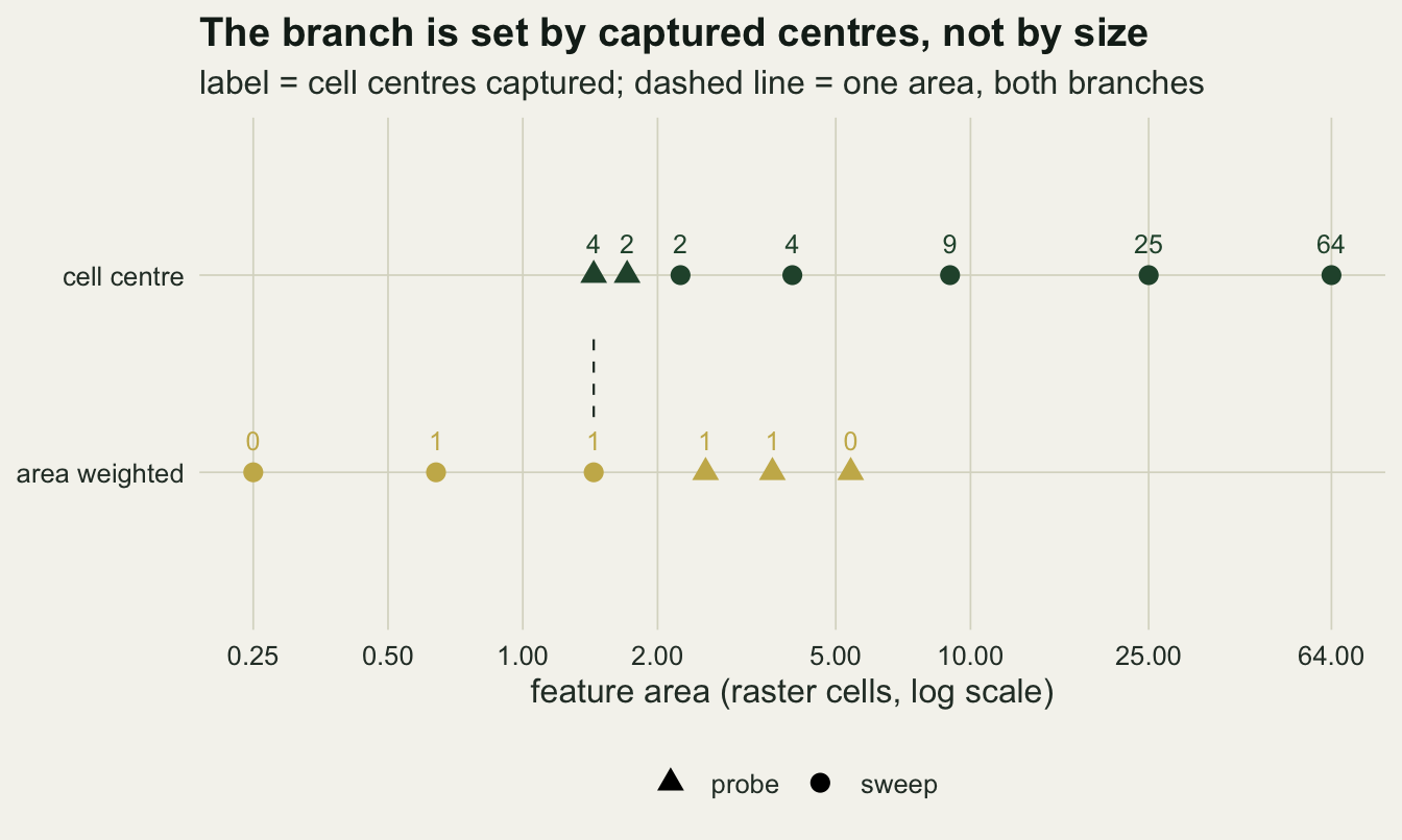
Calling qgis_process from R
If a QGIS step earns its place in a pipeline, it belongs in the script rather than in a note about what was clicked. system2 is enough, and reading --json back gives you the results without parsing prose.
run_qgis <- function(alg, ...) {
  arg <- vapply(list(...), as.character, "")
  out <- system2("qgis_process",
                 c("run", alg, "--json", "--", sprintf("%s=%s", names(arg), arg)),
                 stdout = TRUE, stderr = FALSE)
  jsonlite::fromJSON(paste(out, collapse = "\n"))$results
}
qres <- run_qgis("native:dissolve", INPUT = "patches.gpkg", FIELD = "habitat",
                 OUTPUT = file.path(tempdir(), "dissolved.gpkg"))
dissolved <- st_read(qres$OUTPUT, quiet = TRUE); stopifnot(nrow(dissolved) == 2L)
That chunk is not run when this page is built, and the reason is the argument of the whole section. A pipeline containing it will not run on a machine without QGIS on the path, and this page has to build on one. The stopifnot at the end is the habit worth copying: check the shape of the output rather than the exit status, because the exit status lied in the gdal: failure above.
What to report
Give the QGIS version and the full algorithm identifier, prefix included, for every step that ran through the toolbox. native:buffer and gdal:buffervectors are different programs with different defaults, and a methods section saying “buffered in QGIS” has not said which. Give every parameter you changed, and give the ones you left alone if they move a number. For a buffer that means the segment count, because the QGIS default costs 1.59 per cent of the area of every circle relative to the R default. For a join it means the predicate, the method, and whether unmatched records were discarded. Say which library versions were underneath. Both toolchains print GEOS, GDAL and PROJ on request, qgis_process in its JSON header and sf through sf_extSoftVersion(), and the answer to a geometry question is a property of GEOS at least as much as of the wrapper around it.
For a zonal or raster summary, say which pixels counted, and if the features are small relative to the cell, report how many cell centres they capture rather than how wide they are. On this version that count is what selects the rule: 1 centre or none and the number you are given is area weighted, 2 or more and it is a plain mean over whole cells. A feature that captures one centre and the one beside it that captures two are summarised under different definitions of inside, and they come back in the same column with nothing to mark the difference.
Honest limits
Everything measured here is one QGIS version on one machine. Algorithm identifiers, parameter names and defaults are not stable across major releases: algorithms have been renamed, moved between providers and had their defaults changed, and a script written against one release can fail or, worse, quietly do something else against another. Pinning the QGIS version is not optional if the result has to be reproducible, and that is a heavier dependency than pinning an R package. The switch at 2 captured centres is an empirical rule, fitted to 13 rectangles on one raster under one QGIS build. It is not documented behaviour, it was not read out of the source, and it says nothing about the in place variant of the algorithm or about what happens on a raster that also carries no data cells. What the probes do establish is negative and firmer: neither the width nor the area of the feature predicts the branch, because features of the same width and of the same area sit on both sides.
The comparison was also made easy by both toolchains sitting on the same three libraries, and the QGIS numbers are transcribed. Every command shown was run once in the container and its output copied into a chunk as a literal, so the chunk cannot re-derive them and they carry the trust of a manual step. The sf and terra numbers around them are recomputed wherever this page is built, so a gap in the tenth decimal place of a square metre between two columns is as much a statement about two library builds as about two toolchains. The timing pair is transcribed for the same reason, both halves from the container, and it will not describe a laptop. Anyone repeating this should run the commands rather than take the constants.
The geometry is synthetic, small and rectangular. Rectangles make the captured centre count easy to see and easy to control, which is the whole design of the probe set; a crenulated real boundary captures centres in a way you cannot predict by looking at it, which makes the rule harder to apply but no less operative. The row counts in the join section are specific to this arrangement of twelve circles as well: a denser layer gives a very different ratio of output rows to input features, and that ratio is what surprises people, not the tool.
References
Pebesma E 2018 The R Journal 10(1):439-446 (10.32614/RJ-2018-009)
Bivand RS 2021 Journal of Geographical Systems 23(4):515-546 (10.1007/s10109-020-00336-0)
Steiniger S, Hunter AJS 2013 Computers Environment and Urban Systems 39:136-150 (10.1016/j.compenvurbsys.2012.10.003)
Sandve GK, Nekrutenko A, Taylor J, Hovig E 2013 PLoS Computational Biology 9(10):e1003285 (10.1371/journal.pcbi.1003285)
Hijmans RJ 2023 terra: Spatial Data Analysis. R package version 1.7-65 (https://CRAN.R-project.org/package=terra)