---
title: "From QGIS to R: a spatial join with GeoPackage"
description: "Load occurrence points in QGIS, tag each with the habitat patch it falls in by a spatial join, export to GeoPackage, and continue the analysis in R with sf."
date: "2026-05-04 09:00"
categories: [R, QGIS, sf, spatial, GeoPackage, ecology tutorial]
image: thumbnail.png
image-alt: "Synthetic occurrence points coloured by habitat patch, with points that fall outside every patch shown in grey."
---
A lot of ecological analysis starts in a GUI and finishes in code. You load layers in QGIS, look at them, fix the obvious problems, and then move to R for the statistics. This post walks one small and very common version of that handoff. You have species occurrence points and a set of habitat polygons, and you want every point labelled with the patch it sits inside. QGIS does the looking and the point-in-polygon assignment; R reads the result and summarises it.
The honest framing first: the assignment itself is one line of `sf`. So this is not a case where QGIS does something R cannot. What QGIS gives you here is a place to *see* the data before you trust it, and a searchable catalogue of spatial operations you do not have to remember by name. The post shows both routes and says where each one earns its place.
The screenshots are from QGIS 3.44 LTR. The menu paths are the same in QGIS 4.0, so nothing below goes stale if you are on the newer release.
## The sample data
Everything here runs on synthetic data so you can reproduce it without any field files. The chunk below builds 110 occurrence points spread over a small rectangle of country, plus five habitat polygons. Some points fall outside every polygon on purpose, because a real join almost always leaves a few records unmatched, and handling those is part of the job. It also writes the two files you will open in QGIS: `occurrences.csv` and `habitat_patches.gpkg`. Note that the CSV has no `habitat` column. That column is exactly what the join is about to produce.
```{r}
#| label: make-data
#| message: false
#| warning: false
library(sf)
set.seed(46772359)

# five habitat polygons (lon/lat, EPSG:4326)
mk <- function(m) st_polygon(list(rbind(m, m[1, , drop = FALSE])))
patches <- st_sf(
  patch_id = c("P1", "P2", "P3", "P4", "P5"),
  habitat  = c("forest", "grassland", "wetland", "scrub", "arable"),
  geometry = st_sfc(
    mk(matrix(c(23.520,46.740, 23.570,46.740, 23.570,46.780, 23.520,46.780), ncol = 2, byrow = TRUE)),
    mk(matrix(c(23.580,46.750, 23.630,46.750, 23.630,46.790, 23.580,46.790), ncol = 2, byrow = TRUE)),
    mk(matrix(c(23.550,46.790, 23.600,46.790, 23.600,46.815, 23.550,46.815), ncol = 2, byrow = TRUE)),
    mk(matrix(c(23.635,46.745, 23.685,46.745, 23.685,46.785, 23.635,46.785), ncol = 2, byrow = TRUE)),
    mk(matrix(c(23.515,46.785, 23.550,46.785, 23.550,46.815, 23.515,46.815), ncol = 2, byrow = TRUE)),
    crs = 4326))

# occurrence points: oversample, then keep a controlled mix of inside and outside
cand <- st_as_sf(
  data.frame(lon = runif(2000, 23.50, 23.70), lat = runif(2000, 46.72, 46.82)),
  coords = c("lon", "lat"), crs = 4326, remove = FALSE)
membership <- st_join(cand, patches["habitat"], join = st_intersects)$habitat
inside  <- which(!is.na(membership))
outside <- which(is.na(membership))
keep <- sample(c(sample(inside, 85), sample(outside, 25)))
sel  <- cand[keep, ]
xy   <- st_coordinates(sel)

# species, with a mild habitat preference so there is a signal to find later
inside_hab <- membership[keep]
fav <- list(forest = c("sp1","sp2"), grassland = c("sp3","sp4"), wetland = c("sp5","sp6"),
            scrub = c("sp7","sp8"), arable = c("sp4","sp8"))
spp <- paste0("sp", 1:8)
species <- vapply(seq_along(inside_hab), function(i) {
  if (is.na(inside_hab[i])) return(sample(spp, 1))
  w <- setNames(rep(1, 8), spp); w[fav[[inside_hab[i]]]] <- 4
  sample(spp, 1, prob = w)
}, character(1))

occ <- data.frame(
  site_id   = sprintf("S%03d", seq_along(keep)),
  lon       = round(xy[, 1], 6),
  lat       = round(xy[, 2], 6),
  species   = species,
  abundance = rpois(length(keep), 6) + 1L
)

write.csv(occ, "occurrences.csv", row.names = FALSE)
st_write(patches, "habitat_patches.gpkg", delete_dsn = TRUE, quiet = TRUE)

knitr::kable(head(occ), caption = "First rows of the synthetic occurrence table.")
```
## In QGIS
**1. Load the points.** `Layer` then `Add Layer` then `Add Delimited Text Layer`. Pick `occurrences.csv`, set the format to CSV, choose point geometry with `X field = lon` and `Y field = lat`, and set the geometry CRS to `EPSG:4326 - WGS 84`. The dialog shows you a preview of the table before you commit, which is a good moment to confirm the coordinate columns were read as numbers and not text.
::: {.light-content}
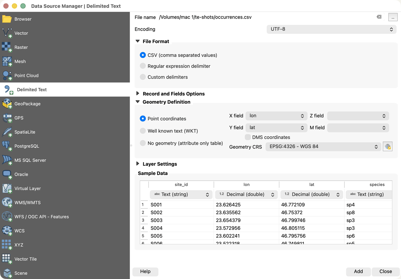{fig-alt="Screenshot of the QGIS Data Source Manager on its Delimited Text page in the light theme. The file name field holds occurrences.csv, the encoding reads UTF-8, and CSV is the chosen file format. Under Geometry Definition, point coordinates is selected with lon in the X field and lat in the Y field, and the geometry CRS reads EPSG:4326 WGS 84. A sample data table below previews the first rows, with site_id read as text and lon and lat read as decimal numbers rather than text. Add and Close buttons sit at the bottom right."}
:::
::: {.dark-content}
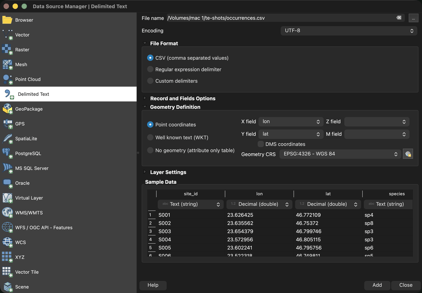{fig-alt="Screenshot of the QGIS Data Source Manager on its Delimited Text page in the dark theme. The file name field holds occurrences.csv, the encoding reads UTF-8, and CSV is the chosen file format. Under Geometry Definition, point coordinates is selected with lon in the X field and lat in the Y field, and the geometry CRS reads EPSG:4326 WGS 84. A sample data table below previews the first rows, with site_id read as text and lon and lat read as decimal numbers rather than text. Add and Close buttons sit at the bottom right."}
:::
**2. Add the polygons and look.** Drag `habitat_patches.gpkg` onto the canvas, or load it through `Add Vector Layer`. Put the point layer above the polygons in the Layers panel. Now you can see the thing you are about to compute: most points land inside a patch, and twenty-five sit outside every one of them. That second group is the reason the join needs a deliberate decision later.
::: {.light-content}
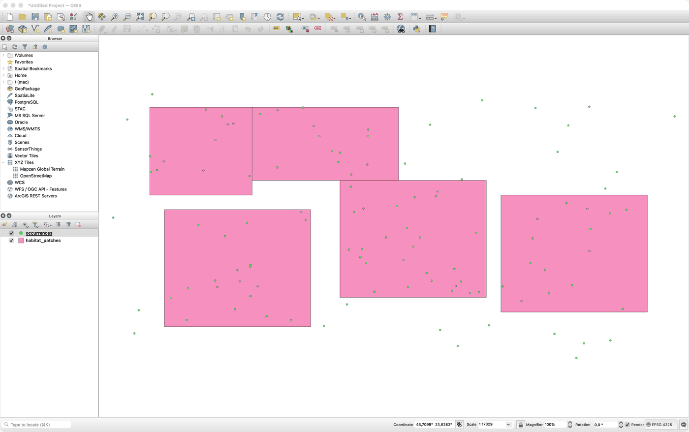{fig-alt="Screenshot of the QGIS main window in the light theme. The Layers panel lists occurrences above habitat_patches. On the canvas five pink rectangles stand for the habitat polygons and small green dots for the occurrence points; most dots sit inside a rectangle and a scatter of them lies in the white space outside every one. The status bar along the bottom shows the cursor coordinate in degrees, a scale of about 1 to 17000, and EPSG:4326 as the project CRS."}
:::
::: {.dark-content}
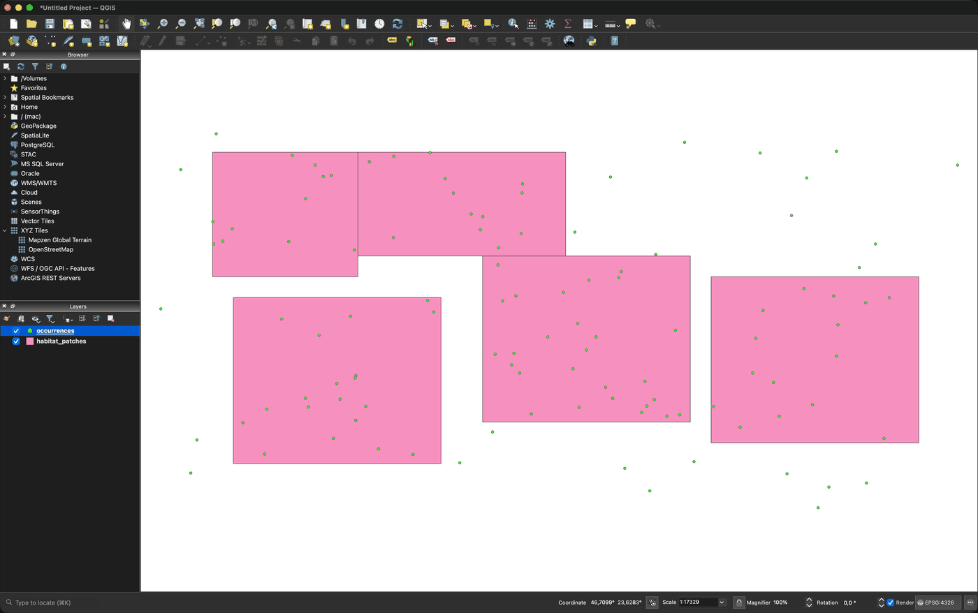{fig-alt="Screenshot of the QGIS main window in the dark theme. The Layers panel lists occurrences above habitat_patches. On the canvas five pink rectangles stand for the habitat polygons and small green dots for the occurrence points; most dots sit inside a rectangle and a scatter of them lies in the white space outside every one. The status bar along the bottom shows the cursor coordinate in degrees, a scale of about 1 to 17000, and EPSG:4326 as the project CRS."}
:::
**3. Move to a projected CRS.** The points came in as longitude and latitude, which is fine for the join but awkward for anything measured in metres. Open `Project` then `Properties` then `CRS` (or click the CRS button at the bottom right of the window), filter for `3844`, and choose `EPSG:3844 - Pulkovo 1942(58) / Stereo70`, the national projected system for Romania. The map reprojects on the fly. A spatial join by intersection gives the same answer in either CRS, but working in metres keeps distances and areas honest once you start measuring things.
::: {.light-content}
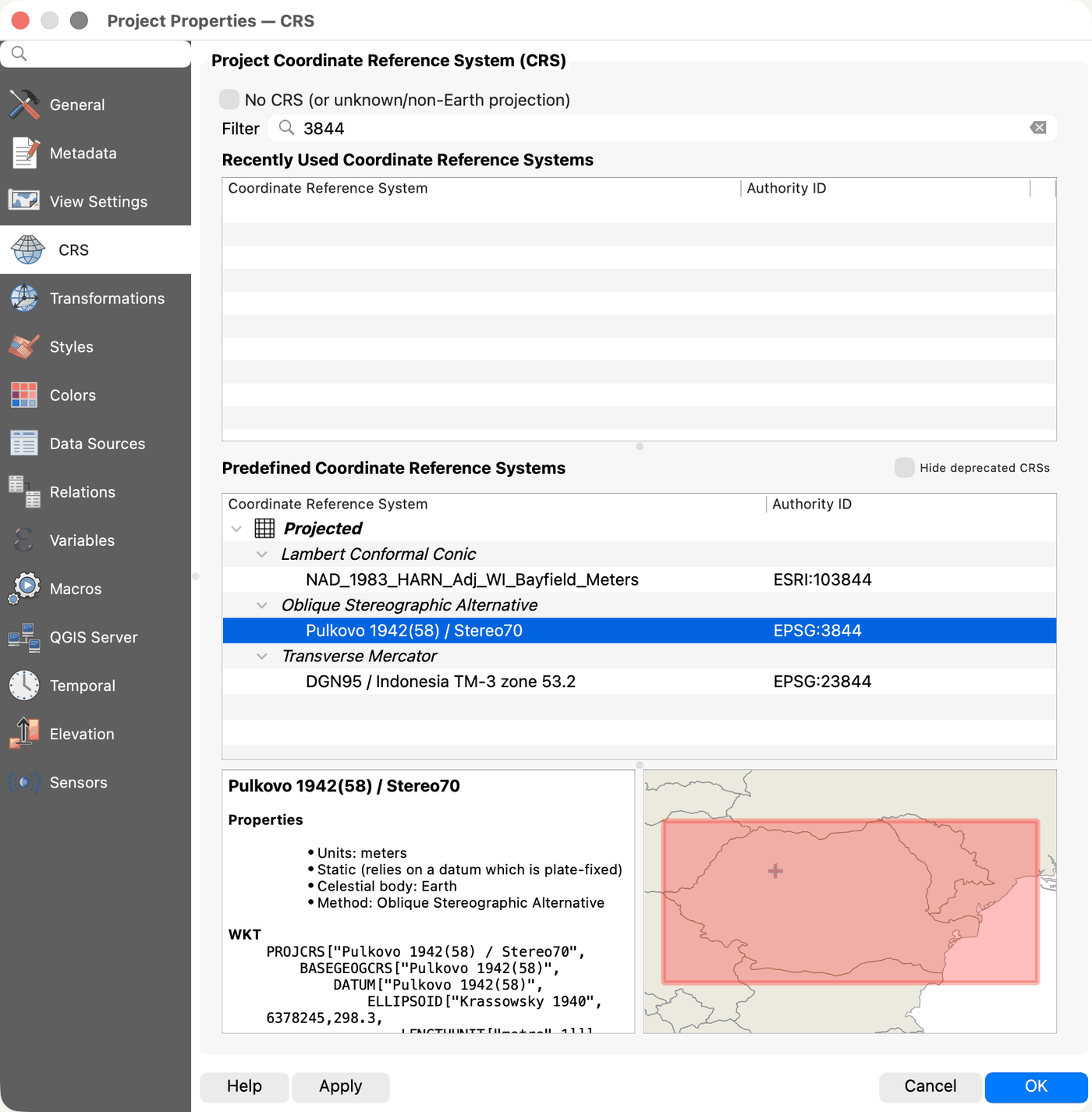{fig-alt="Screenshot of the QGIS Project Properties window on its CRS page in the light theme. The filter box holds 3844 and the recently used list is empty. In the predefined list, Pulkovo 1942(58) / Stereo70 with authority ID EPSG:3844 is highlighted under Oblique Stereographic Alternative, between a Lambert Conformal Conic entry and a Transverse Mercator entry that also match the filter. A properties panel below gives the units as metres and the method as Oblique Stereographic Alternative, followed by the start of the WKT definition, and a small map to its right shades the area of use over Romania."}
:::
::: {.dark-content}
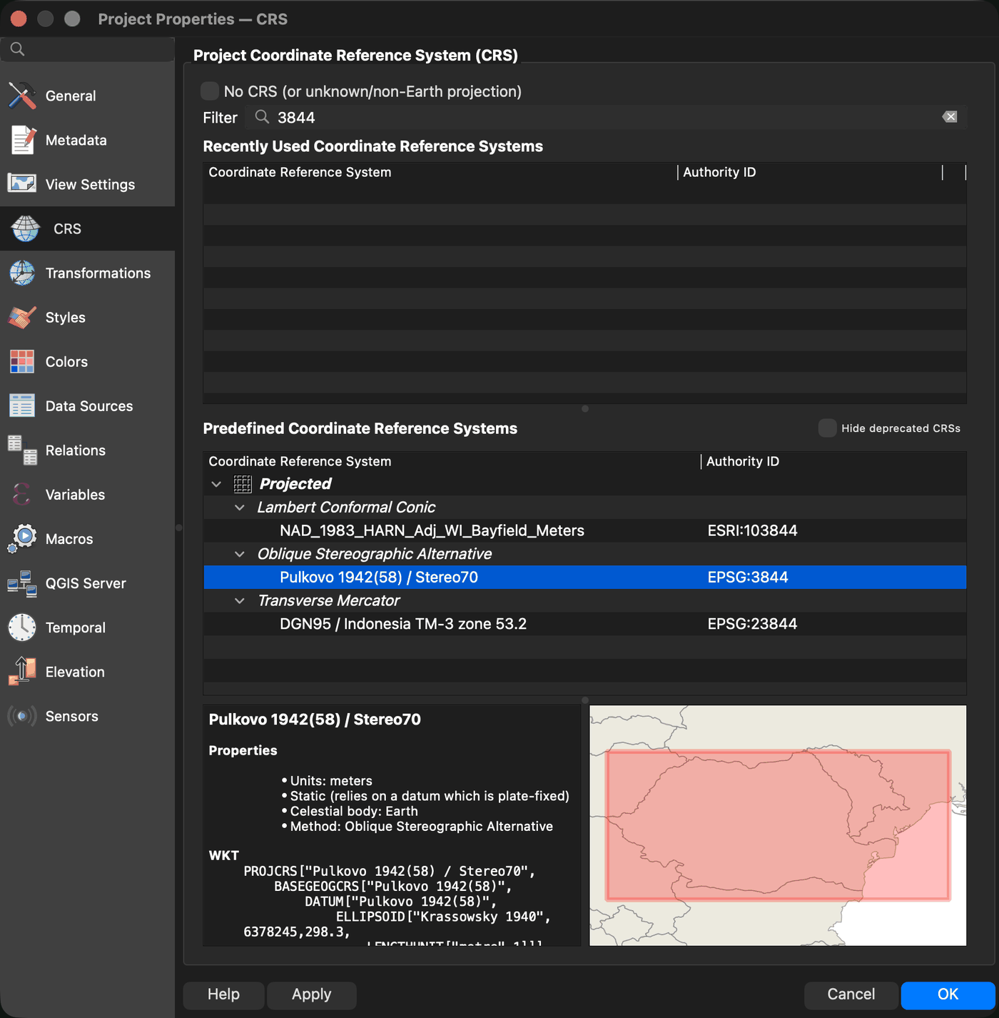{fig-alt="Screenshot of the QGIS Project Properties window on its CRS page in the dark theme. The filter box holds 3844 and the recently used list is empty. In the predefined list, Pulkovo 1942(58) / Stereo70 with authority ID EPSG:3844 is highlighted under Oblique Stereographic Alternative, between a Lambert Conformal Conic entry and a Transverse Mercator entry that also match the filter. A properties panel below gives the units as metres and the method as Oblique Stereographic Alternative, followed by the start of the WKT definition, and a small map to its right shades the area of use over Romania."}
:::
**4. Run the spatial join.** Open `Processing` then `Toolbox`, and search for `Join attributes by location`. Set the base layer to `occurrences` and the join layer to `habitat_patches`. Use the `intersects` predicate, and a join type of *take attributes of the first matching feature only*, since each point sits in at most one patch. Leave `Discard records which could not be joined` unchecked. That box is the whole decision: unchecked, the 25 outside points stay in the output with an empty `habitat`, which is what you want so you can account for them rather than lose them silently.
::: {.light-content}
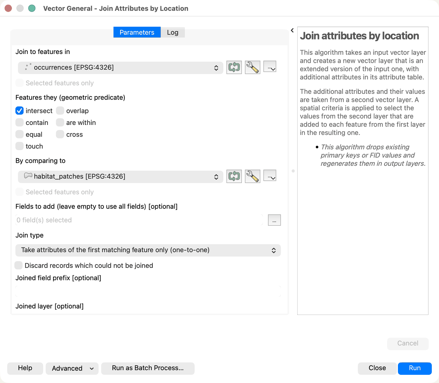{fig-alt="Screenshot of the QGIS Join attributes by location dialog in the light theme, its title bar reading Vector General. The base layer field holds occurrences EPSG:4326 and the comparison field holds habitat_patches EPSG:4326. Of the seven geometric predicates only intersect is ticked. Fields to add reads 0 fields selected, the join type reads take attributes of the first matching feature only one-to-one, and the discard records which could not be joined box is unticked. A help panel on the right describes the algorithm, and Close and Run buttons sit at the bottom right."}
:::
::: {.dark-content}
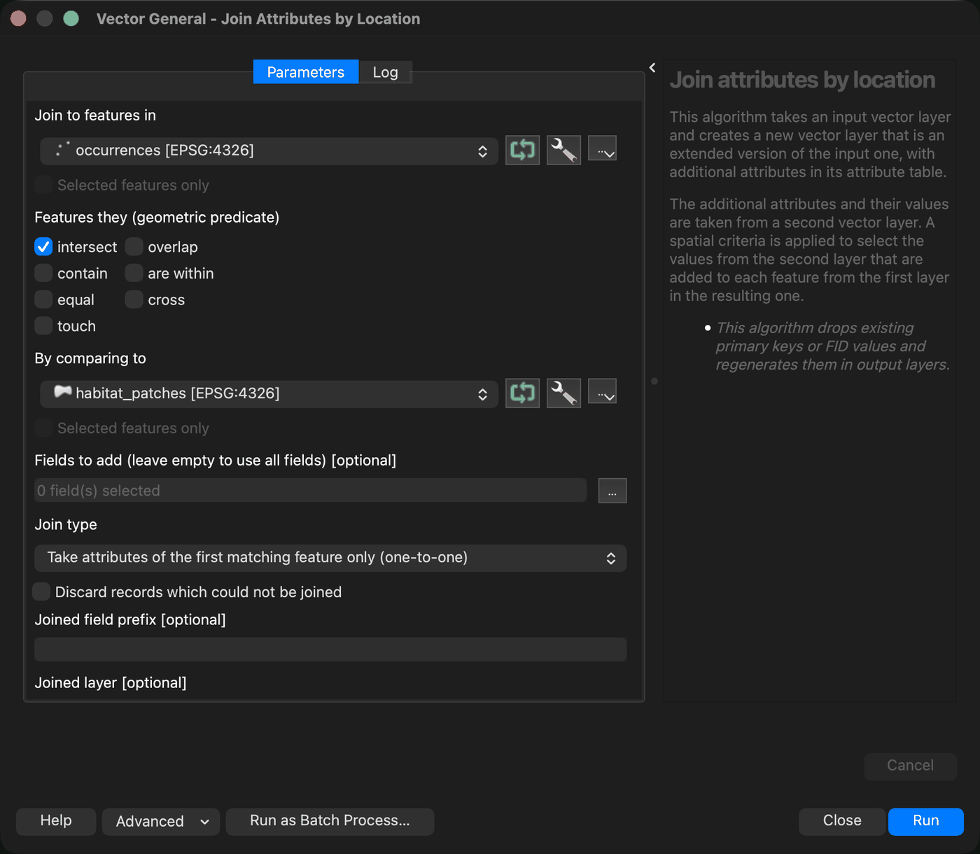{fig-alt="Screenshot of the QGIS Join attributes by location dialog in the dark theme, its title bar reading Vector General. The base layer field holds occurrences EPSG:4326 and the comparison field holds habitat_patches EPSG:4326. Of the seven geometric predicates only intersect is ticked. Fields to add reads 0 fields selected, the join type reads take attributes of the first matching feature only one-to-one, and the discard records which could not be joined box is unticked. A help panel on the right describes the algorithm, and Close and Run buttons sit at the bottom right."}
:::
**5. Export to GeoPackage.** Right-click the joined layer, then `Export` then `Save Features As`. Choose GeoPackage as the format, name the file `occurrences_joined.gpkg`, and set the output CRS to `EPSG:3844`. GeoPackage is the clean way to hand vector data to R: one file, an open OGC standard, and none of the four-file shapefile baggage. That single file is the entire handoff.
## Back in R
QGIS wrote `occurrences_joined.gpkg`, and you can read it straight back:
```{r}
#| label: read-gpkg
#| eval: false
library(sf)
occ_tagged <- st_read("occurrences_joined.gpkg")
```
To keep this post reproducible without anyone repeating the clicks, here is the same point-in-polygon assignment as the single `sf` call it really is. This is what the figures below use, and it returns the same labels QGIS produced:
```{r}
#| label: join
occ_sf <- st_as_sf(occ, coords = c("lon", "lat"), crs = 4326)
occ_tagged <- st_join(occ_sf, patches["habitat"], join = st_intersects)
occ_tagged$habitat[is.na(occ_tagged$habitat)] <- "unassigned"

table(occ_tagged$habitat)
```
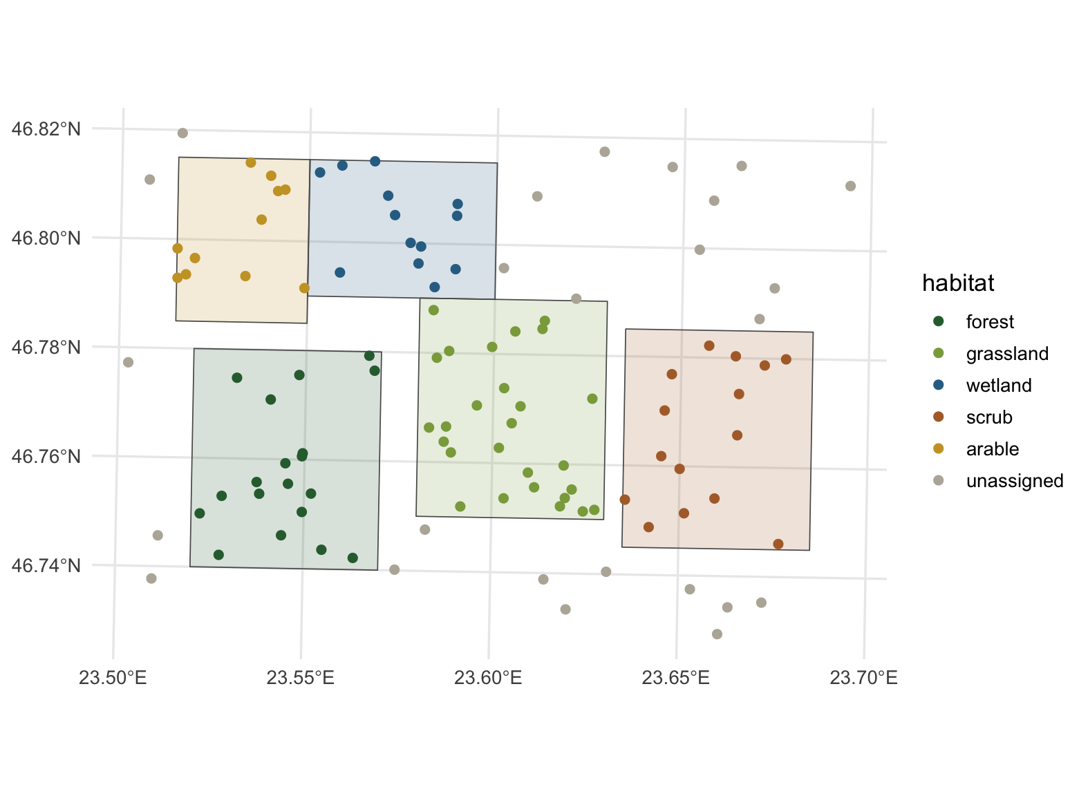
The 25 points outside every patch now carry the label `unassigned` instead of a missing value, which keeps them visible in summaries. Here is the joined result drawn in R, projected to Stereo70:
```{r}
#| label: fig-map
#| message: false
#| warning: false
#| fig-width: 8.2
#| fig-height: 6
#| fig-cap: "The joined points, coloured by the habitat patch each one falls in. Grey points lie outside every patch."
#| fig-alt: "A map of occurrence points over five habitat polygons. Points are coloured by habitat; points outside any polygon are grey."
library(ggplot2)
te_canvas <- theme(plot.background  = element_rect(fill = "#f5f4ee", colour = NA),
                   panel.background = element_rect(fill = "#f5f4ee", colour = NA))
hab_levels <- c("forest", "grassland", "wetland", "scrub", "arable", "unassigned")
hab_cols <- c(forest = "#2f6b3c", grassland = "#8aa84b", wetland = "#2f6f93",
              scrub = "#b06d35", arable = "#caa12e", unassigned = "#b8b3a7")

occ_3844     <- st_transform(occ_tagged, 3844)
patches_3844 <- st_transform(patches, 3844)
occ_3844$habitat     <- factor(occ_3844$habitat, levels = hab_levels)
patches_3844$habitat <- factor(patches_3844$habitat, levels = hab_levels)

ggplot() +
  geom_sf(data = patches_3844, aes(fill = habitat), colour = "grey35", linewidth = 0.3, alpha = 0.18) +
  geom_sf(data = occ_3844, aes(colour = habitat), size = 2) +
  scale_fill_manual(values = hab_cols, drop = FALSE, guide = "none") +
  scale_colour_manual(values = hab_cols, drop = FALSE, name = "habitat") +
  labs(x = NULL, y = NULL) +
  theme_minimal(base_size = 13) + te_canvas +
  theme(panel.grid = element_line(colour = "grey92"))
```
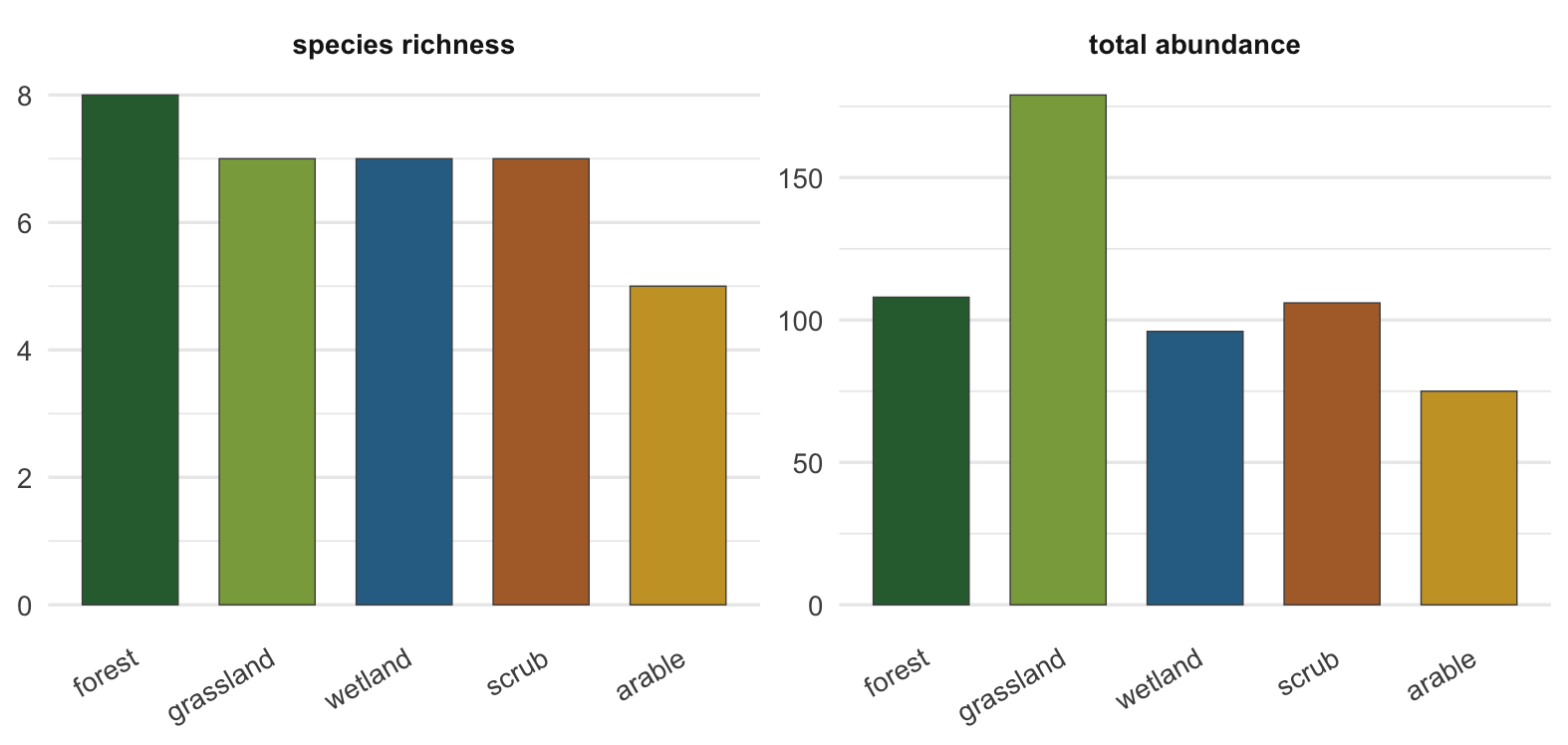
With a `habitat` column attached, the kind of summary you came for is now ordinary data work. Counting species richness and total abundance per habitat takes a single grouped summary:
```{r}
#| label: summary
#| message: false
#| warning: false
library(dplyr)
per_habitat <- occ_tagged |>
  st_drop_geometry() |>
  filter(habitat != "unassigned") |>
  group_by(habitat) |>
  summarise(richness = n_distinct(species),
            total_abundance = sum(abundance),
            records = n(),
            .groups = "drop")

knitr::kable(per_habitat, caption = "Richness and abundance per habitat, after the join.")
```
```{r}
#| label: fig-summary
#| message: false
#| warning: false
#| fig-width: 8.2
#| fig-height: 3.9
#| fig-cap: "Species richness and total abundance per habitat for the matched points."
#| fig-alt: "Two bar panels. The left panel shows species richness per habitat; the right panel shows total abundance per habitat."
library(tidyr)
per_habitat |>
  pivot_longer(c(richness, total_abundance), names_to = "metric", values_to = "value") |>
  mutate(metric = factor(metric, c("richness", "total_abundance"),
                         c("species richness", "total abundance")),
         habitat = factor(habitat, hab_levels)) |>
  ggplot(aes(habitat, value, fill = habitat)) +
  geom_col(width = 0.7, colour = "grey30", linewidth = 0.25) +
  facet_wrap(~ metric, scales = "free_y") +
  scale_fill_manual(values = hab_cols, drop = FALSE, guide = "none") +
  labs(x = NULL, y = NULL) +
  theme_minimal(base_size = 13) + te_canvas +
  theme(panel.grid.major.x = element_blank(),
        axis.text.x = element_text(angle = 30, hjust = 1),
        strip.text = element_text(face = "bold"))
```
## Which tool, when
A spatial join is a fair test of where the line sits. In `sf` it is one call, it is scripted, and it drops straight into a pipeline, so for anything you want to rerun or version it belongs in R. QGIS earns its place just before that: it is where you confirm the points landed where they should, where you catch the ones that fell in the sea because a CRS was set wrong, and where you reach for an operation by browsing the toolbox instead of recalling its name. The GeoPackage is what keeps the two honest with each other, a single standardised file passed from the place you looked at the data to the place you analyse it.
## References
Pebesma E 2018 The R Journal 10(1):439-446 (10.32614/RJ-2018-009)
## Related tutorials
- [Raster basics with terra](../terra-raster-basics/)
- [QGIS NULL and R NA: what survives the trip](../qgis-null-and-r-na/)
- [Richness mapping with sf](../richness-mapping-sf/)
- [Running QGIS from the command line](../running-qgis-from-the-command-line/)