library(sf)
library(dplyr)
library(ggplot2)
te_paper <- "#f5f4ee"; te_ink <- "#16241d"; te_body <- "#2c3a31"
te_forest <- "#275139"; te_rust <- "#b5534e"; te_gold <- "#c9b458"
te_line <- "#dad9ca"
theme_datasheet <- function() theme_minimal(base_size = 12) +
theme(plot.background = element_rect(fill = te_paper, colour = NA), panel.grid.minor = element_blank(),
panel.grid.major = element_line(colour = te_line, linewidth = 0.3),
text = element_text(colour = te_body), axis.text = element_text(colour = te_body),
plot.title = element_text(colour = te_ink, face = "bold"))
# how a value is shown in the tables below: NULL for a missing value, '' for empty text
show_val <- function(v) ifelse(is.na(v), "NULL", ifelse(v == "", "''", as.character(v)))
tick <- function(x) paste0("\x60", x, "\x60") # a value shown as inline code in the text
show_md <- function(v) { s <- show_val(v); ifelse(s %in% c("NULL", "''"), paste0("`", s, "`"), s) }
# an expression inside an HTML code tag, so a pipe cannot split the table and quotes stay straight
code_cell <- function(x) {
x <- gsub("&", "&", x, fixed = TRUE); x <- gsub("|", "|", x, fixed = TRUE)
x <- gsub("\"", """, x, fixed = TRUE); x <- gsub("'", "'", x, fixed = TRUE)
paste0("<code>", gsub("<", "<", x, fixed = TRUE), "</code>")
}QGIS NULL and R NA: what survives the trip
R
QGIS
sf
GeoPackage
missing data
data management
ecology tutorial
QGIS NULL and R NA agree on comparisons and filters, but not on bare [ indexing, aggregates or pasted text, and a CSV export merges NULL with empty text.
A vegetation survey of forty plots comes back from the field as a point layer. Every plot should carry a habitat class and the percentage cover of the dominant shrub. Five plots were never reached, so nobody entered a habitat for them, and the QGIS attribute table shows the word NULL in that cell. Three more were visited, but their habitat cell holds an empty piece of text, which is what a merged spreadsheet or a cleared form field tends to leave behind. The table shows those three as empty cells. The two cases mean different things: not recorded, and recorded as nothing. Six plots also have no cover value.
Then the same question gets asked twice. How many plots are not forest? QGIS answers with one count and R, reading the same file, can answer with another; after a CSV export the eight habitat gaps can no longer be told apart at all. Reading field data into R covers the R half of the missing value story: read.csv turns an empty field into NA in a numeric column and into an empty string in a text column, and na.strings is where you declare your own codes. What a shapefile loses follows attribute types through a shapefile, and From QGIS to R: a spatial join with GeoPackage walks the ordinary GeoPackage handoff. This post covers the missing values on the QGIS side of that handoff: what a QGIS expression does with NULL, which R call does the same thing with NA, and which export format keeps NULL apart from the empty string.
The QGIS numbers come from QGIS 3.34.4 on Linux, run headless through qgis_process as in Running QGIS from the command line, plus one short PyQGIS script. Nothing on this page calls QGIS when it is built. Each command is shown in a plain block, exactly as it was run from this post’s folder, and what it wrote is saved as a small file next to the page; the R chunks read those files. The two input layers are written by the R chunks below, so the chain runs R, then QGIS, then R. Where a step has a desktop equivalent, the menu path is given in bold, checked against the QGIS 3.40 user manual.
Six plots you can read whole
Before the forty plots, six, small enough to check every cell by eye. The table uses the QGIS convention of writing a missing value as NULL, and writes the empty string as two quote marks so it can be seen.
six <- st_sf(
  plot_id  = 1:6,
  habitat  = c("forest", "grassland", NA, "", "forest", "wetland"),
  cover    = c(80, 20, NA, 35, NA, 60),
  geometry = st_sfc(lapply(1:6, function(i) st_point(c(23.55 + i / 100, 46.75))), crs = 4326))
st_write(six, "six-plots.gpkg", delete_dsn = TRUE, quiet = TRUE)
six_tab <- st_drop_geometry(six)
knitr::kable(data.frame(plot_id = six_tab$plot_id, habitat = show_md(six_tab$habitat),
                        cover = show_md(six_tab$cover)),
caption = "The six plot layer as written to six-plots.gpkg.")| plot_id | habitat | cover |
|---|---|---|
| 1 | forest | 80 |
| 2 | grassland | 20 |
| 3 | NULL |
NULL |
| 4 | '' |
35 |
| 5 | forest | NULL |
| 6 | wetland | 60 |
Plot 3 was not recorded at all. Plot 4 was recorded with an empty habitat. Plot 5 has a habitat but no cover. In R the first is NA, the second is "", and sf writes them to the GeoPackage as a SQL NULL and as a zero length text value, which is what QGIS reads.
What an expression does with NULL
The desktop tool is the Field Calculator (the Open field calculator button on the attribute table toolbar, Ctrl+I there), or its Processing twin under Processing > Toolbox > Vector table > Field calculator. The twin is the one that runs from the command line. The block below adds eleven fields to a copy of the layer, one expression per field, each call reading the previous call’s output. The type codes are the algorithm’s own: 6 is boolean, 0 decimal, 1 integer, 2 text.
export QT_QPA_PLATFORM=offscreen
calc() {  # add one field to the running copy: name, type code, expression
  qgis_process run native:fieldcalculator -- INPUT=calc-in.gpkg FIELD_NAME="$1" \
    FIELD_TYPE="$2" FORMULA="$3" OUTPUT=calc-out.gpkg > /dev/null
  mv calc-out.gpkg calc-in.gpkg
}
cp six-plots.gpkg calc-in.gpkg
calc ne_forest    6 "\"habitat\" != 'forest'"
calc isnot_forest 6 "\"habitat\" IS NOT 'forest'"
calc is_null      6 "\"habitat\" IS NULL"
calc is_blank     6 "\"habitat\" = ''"
calc cover_x2     0 "\"cover\" * 2"
calc mean_cover   0 "mean(\"cover\")"
calc count_cover  1 "count(\"cover\")"
calc miss_cover   1 "count_missing(\"cover\")"
calc pipe_x       2 "\"habitat\" || '_x'"
calc concat_x     2 "concat(\"habitat\", '_x')"
calc filled       2 "coalesce(\"habitat\", 'not recorded')"
mv calc-in.gpkg six-plots-calc.gpkg
The chunk below reads six-plots-calc.gpkg back and sets each QGIS column beside the R expression that ought to match it. Where the obvious R call does not match, the table carries both: the obvious one and the one that does.
qc  <- st_drop_geometry(st_read("six-plots-calc.gpkg", quiet = TRUE))
hab <- six_tab$habitat; cov <- six_tab$cover
fmt_q <- function(v) code_cell(paste(show_val(v), collapse = " "))
fmt_r <- function(v) code_cell(paste(ifelse(is.na(v), "NA", show_val(v)), collapse = " "))
pairs <- list(
  list("\"habitat\" != 'forest'", "habitat != \"forest\"", qc$ne_forest, hab != "forest"),
  list("\"habitat\" IS NOT 'forest'", "!(habitat %in% \"forest\")", qc$isnot_forest,
       !(hab %in% "forest")),
  list("\"habitat\" IS NULL", "is.na(habitat)", qc$is_null, is.na(hab)),
  list("\"habitat\" = ''", "habitat == \"\"", qc$is_blank, hab == ""),
  list("\"cover\" * 2", "cover * 2", qc$cover_x2, cov * 2),
  list("mean(\"cover\")", "mean(cover)", unique(qc$mean_cover), mean(cov)),
  list("mean(\"cover\")", "mean(cover, na.rm = TRUE)", unique(qc$mean_cover),
       mean(cov, na.rm = TRUE)),
  list("count(\"cover\")", "sum(!is.na(cover))", unique(qc$count_cover), sum(!is.na(cov))),
  list("count_missing(\"cover\")", "sum(is.na(cover))", unique(qc$miss_cover), sum(is.na(cov))),
  list("\"habitat\" || '_x'", "paste0(habitat, \"_x\")", qc$pipe_x, paste0(hab, "_x")),
  list("\"habitat\" || '_x'", "ifelse(is.na(habitat), NA, paste0(habitat, \"_x\"))",
       qc$pipe_x, ifelse(is.na(hab), NA, paste0(hab, "_x"))),
  list("concat(\"habitat\", '_x')", "paste0(coalesce(habitat, \"\"), \"_x\")", qc$concat_x,
       paste0(coalesce(hab, ""), "_x")),
  list("coalesce(\"habitat\", 'not recorded')", "coalesce(habitat, \"not recorded\")",
       qc$filled, coalesce(hab, "not recorded")))
corr <- data.frame(
  QGIS = vapply(pairs, function(p) code_cell(p[[1]]), ""),
  R    = vapply(pairs, function(p) code_cell(p[[2]]), ""),
  QGIS_result = vapply(pairs, function(p) fmt_q(p[[3]]), ""),
  R_result    = vapply(pairs, function(p) fmt_r(p[[4]]), ""),
  same = vapply(pairs, function(p) identical(show_val(p[[3]]), show_val(p[[4]])), TRUE))
knitr::kable(corr, escape = FALSE, row.names = FALSE,
caption = "One QGIS expression and one R expression per row, on plots 1 to 6. QGIS results print a missing value as NULL, R results as NA.")| QGIS | R | QGIS_result | R_result | same |
|---|---|---|---|---|
"habitat" != 'forest' |
habitat != "forest" |
FALSE TRUE NULL TRUE FALSE TRUE |
FALSE TRUE NA TRUE FALSE TRUE |
TRUE |
"habitat" IS NOT 'forest' |
!(habitat %in% "forest") |
FALSE TRUE TRUE TRUE FALSE TRUE |
FALSE TRUE TRUE TRUE FALSE TRUE |
TRUE |
"habitat" IS NULL |
is.na(habitat) |
FALSE FALSE TRUE FALSE FALSE FALSE |
FALSE FALSE TRUE FALSE FALSE FALSE |
TRUE |
"habitat" = '' |
habitat == "" |
FALSE FALSE NULL TRUE FALSE FALSE |
FALSE FALSE NA TRUE FALSE FALSE |
TRUE |
"cover" * 2 |
cover * 2 |
160 40 NULL 70 NULL 120 |
160 40 NA 70 NA 120 |
TRUE |
mean("cover") |
mean(cover) |
48.75 |
NA |
FALSE |
mean("cover") |
mean(cover, na.rm = TRUE) |
48.75 |
48.75 |
TRUE |
count("cover") |
sum(!is.na(cover)) |
4 |
4 |
TRUE |
count_missing("cover") |
sum(is.na(cover)) |
2 |
2 |
TRUE |
"habitat" || '_x' |
paste0(habitat, "_x") |
forest_x grassland_x NULL _x forest_x wetland_x |
forest_x grassland_x NA_x _x forest_x wetland_x |
FALSE |
"habitat" || '_x' |
ifelse(is.na(habitat), NA, paste0(habitat, "_x")) |
forest_x grassland_x NULL _x forest_x wetland_x |
forest_x grassland_x NA _x forest_x wetland_x |
TRUE |
concat("habitat", '_x') |
paste0(coalesce(habitat, ""), "_x") |
forest_x grassland_x _x _x forest_x wetland_x |
forest_x grassland_x _x _x forest_x wetland_x |
TRUE |
coalesce("habitat", 'not recorded') |
coalesce(habitat, "not recorded") |
forest grassland not recorded '' forest wetland |
forest grassland not recorded '' forest wetland |
TRUE |
n_pairs <- nrow(corr); n_same <- sum(corr$same)
q_mean  <- unique(qc$mean_cover); q_count <- unique(qc$count_cover); q_miss <- unique(qc$miss_cover)
r_paste <- paste0(hab, "_x")[3]
11 of the 13 pairs match cell for cell. The first four rows are the three-valued logic the two tools share. A comparison with a missing value has no answer, so "habitat" != 'forest' on plot 3 is NULL in QGIS, and habitat != "forest" is NA in R, in the same row. "habitat" = '' is NULL there too, which is why NULL and the empty string never catch each other: IS NULL finds plot 3 only, = '' finds plot 4 only. The fix in QGIS for a comparison that should see NULL as a value is IS and IS NOT, which the manual defines as “the same as” and which, as the plot 3 value in the IS NOT row shows, return true or false even when one side is NULL; the R twin is %in%, which never returns NA. Arithmetic behaves the same in both tools: a missing input gives a missing output.
The two tools part company over what happens by default. mean("cover") in QGIS is 48.75, averaged over the 4 plots that have a cover value, and count("cover") counts only those; count_missing("cover") gives the 2 it left out. Aggregates in QGIS skip NULL without saying so. mean(cover) in R is NA and stays NA until you pass na.rm = TRUE, at which point the two agree. Neither default is wrong, but a QGIS mean pasted into a report next to an R mean of the same column can differ for this reason alone.
Text is where the differences are least visible. The || operator returns NULL if either side is NULL, and the manual says so. concat() converts NULL to an empty string first, so plot 3 comes out as _x, exactly like plot 4, and the NULL has been erased from the new field. R adds a third behaviour: paste0() turns NA into the two letters N and A, so plot 3 becomes NA_x, a habitat class nobody recorded. coalesce() replaces NULL and nothing else, so the recorded blank on plot 4 stays blank.
A filter keeps what is true and nothing else
Now the forty plots, with the design fixed in the chunk below (habitat counts and missing cover set in advance, shuffled with a seed).
set.seed(20261011)
n_plot   <- 40
hab_pool <- rep(c("forest", "grassland", "wetland", "scrub", NA, ""), c(14, 9, 6, 3, 5, 3))
survey <- st_sf(
  plot_id  = seq_len(n_plot),
  habitat  = sample(hab_pool),
  cover    = round(runif(n_plot, 5, 95)),
  geometry = st_sfc(lapply(seq_len(n_plot), function(i)
    st_point(c(23.55 + runif(1, 0, 0.08), 46.74 + runif(1, 0, 0.06)))), crs = 4326))
survey$cover[sample(n_plot, 6)] <- NA
st_write(survey, "survey-plots.gpkg", delete_dsn = TRUE, quiet = TRUE)
n_forest <- sum(survey$habitat %in% "forest"); n_null <- sum(is.na(survey$habitat))
n_blank  <- sum(survey$habitat %in% ""); n_cover_na <- sum(is.na(survey$cover))
n_other  <- n_plot - n_forest - n_null - n_blank
The question is how many plots are not forest. In the desktop that is Processing > Toolbox > Vector selection > Extract by expression, or Edit > Select > Select Features by Expression (Ctrl+F3), which evaluates the same expression; the PyQGIS script in the export section runs that selection on this layer and saves its counts to qgis-select.csv. Extract by expression can also write the features that did not match to a second output, and that output is the more revealing of the two. Only the plot_id column of the four output files is used, so their being CSV does not matter yet.
qgis_process run native:extractbyexpression -- INPUT=survey-plots.gpkg \
  EXPRESSION="\"habitat\" != 'forest'" OUTPUT=qgis-ne-forest.csv FAIL_OUTPUT=qgis-ne-forest-fail.csv
qgis_process run native:extractbyexpression -- INPUT=survey-plots.gpkg \
  EXPRESSION="\"habitat\" IS NOT 'forest'" OUTPUT=qgis-isnot-forest.csv
qgis_process run native:extractbyexpression -- INPUT=survey-plots.gpkg \
  EXPRESSION="\"habitat\" IS NULL" OUTPUT=qgis-is-null.csv
qgis_process run native:extractbyexpression -- INPUT=survey-plots.gpkg \
  EXPRESSION="\"habitat\" = ''" OUTPUT=qgis-is-blank.csv
q_ids <- function(f) read.csv(f)$plot_id
# names are markdown code spans for the table (a bare $ would start TeX math); the figure drops the backticks
ids <- list(
"QGIS: `\"habitat\" != 'forest'`" = q_ids("qgis-ne-forest.csv"),
"QGIS: the same, non-matching output" = q_ids("qgis-ne-forest-fail.csv"),
"QGIS: `\"habitat\" IS NOT 'forest'`" = q_ids("qgis-isnot-forest.csv"),
"R: `filter(x, habitat != \"forest\")`" = filter(survey, habitat != "forest")$plot_id,
"R: `subset(x, habitat != \"forest\")`" = subset(survey, habitat != "forest")$plot_id,
"R: `x[x$habitat != \"forest\", ]`" = survey[survey$habitat != "forest", ]$plot_id,
"R: `x[which(x$habitat != \"forest\"), ]`" = survey[which(survey$habitat != "forest"), ]$plot_id,
"R: `x[!(x$habitat %in% \"forest\"), ]`" = survey[!(survey$habitat %in% "forest"), ]$plot_id)
kind_of <- function(id) {
h <- survey$habitat[match(id, survey$plot_id)]
ifelse(is.na(id), "row of NA", ifelse(is.na(h), "not recorded (NULL)",
ifelse(h == "", "empty text", ifelse(h == "forest", "forest", "other habitat"))))
}
filt <- data.frame(formulation = names(ids), rows = lengths(ids),
not_recorded = vapply(ids, function(z) sum(kind_of(z) == "not recorded (NULL)"), 0L),
rows_of_NA = vapply(ids, function(z) sum(is.na(z)), 0L), row.names = NULL)
knitr::kable(filt, caption = "Rows returned from the forty plot survey by each way of asking for plots that are not forest.")| formulation | rows | not_recorded | rows_of_NA |
|---|---|---|---|
QGIS: "habitat" != 'forest' |
21 | 0 | 0 |
| QGIS: the same, non-matching output | 19 | 5 | 0 |
QGIS: "habitat" IS NOT 'forest' |
26 | 5 | 0 |
R: filter(x, habitat != "forest") |
21 | 0 | 0 |
R: subset(x, habitat != "forest") |
21 | 0 | 0 |
R: x[x$habitat != "forest", ] |
26 | 0 | 5 |
R: x[which(x$habitat != "forest"), ] |
21 | 0 | 0 |
R: x[!(x$habitat %in% "forest"), ] |
26 | 5 | 0 |
n_q_ne   <- length(ids[[1]]); n_q_fail <- length(ids[[2]]); n_q_isnot <- length(ids[[3]])
n_filter <- length(ids[[4]]); n_bracket <- length(ids[[6]]); n_na_rows <- sum(is.na(ids[[6]]))
same_filter <- identical(sort(ids[[1]]), sort(ids[[4]])) && identical(sort(ids[[1]]), sort(ids[[5]])) &&
  identical(sort(ids[[1]]), sort(ids[[7]]))
same_isnot  <- identical(sort(ids[[3]]), sort(ids[[8]]))
na_rows_empty <- all(st_is_empty(survey[survey$habitat != "forest", ])[is.na(ids[[6]])])
n_blank_bracket <- nrow(survey[survey$habitat == "", ])
n_q_null <- length(q_ids("qgis-is-null.csv")); n_q_blank <- length(q_ids("qgis-is-blank.csv"))
fail_kind <- kind_of(ids[[2]]); n_fail_forest <- sum(fail_kind == "forest")
n_fail_null <- sum(fail_kind == "not recorded (NULL)"); n_ne_null <- filt$not_recorded[1]
sel <- read.csv("qgis-select.csv")
sel_ne <- sel$selected[sel$test == "ne_forest"]; sel_isnot <- sel$selected[sel$test == "isnot_forest"]
The survey has 18 plots of another habitat, 3 with empty text, 5 not recorded and 14 forest, and 6 plots without a cover value. QGIS returns 21 plots for "habitat" != 'forest': the other habitats and the empty text. The number of unrecorded plots among them is 0; they sit in the non-matching output instead, which holds 19 plots: 14 forest plots and the 5 nobody visited, filed together as if they were forest. The reason is the NULL that != returned for plot 3 in the six plot table. A filter keeps a feature when the expression is true, and NULL is not true, so it goes wherever false goes.
dplyr::filter() and subset() follow the same rule and say so in their help pages: a condition that evaluates to NA drops the row. Both return the same 21 plots as QGIS, whose selection tool also picks 21, and a check that the plot sets are identical, which() included, returns TRUE. Square bracket indexing does not follow that rule. An NA index, in the words of ?Extract, “picks an unknown element”, and for a data frame R answers with a row in which every column is NA: no plot number, no habitat, no cover, and an empty point for a geometry. x[x$habitat != "forest", ] therefore returns 26 rows, of which 5 are these rows of NA and not plots at all (their geometries are all empty: TRUE). nrow() counts them, and so does any tally of records made from that object. The same thing happens with the empty text: x[x$habitat == "", ] gives 8 rows for 3 blank plots.
If the unrecorded plots are wanted in the answer, say so. "habitat" IS NOT 'forest' in QGIS returns 26 plots (the selection tool: 26), and !(habitat %in% "forest") in R returns the same plots (TRUE), unrecorded ones included and 0 rows of NA.
filt_long <- do.call(rbind, lapply(names(ids), function(k)
  data.frame(formulation = gsub("`", "", k), kind = kind_of(ids[[k]]))))
filt_long$formulation <- factor(filt_long$formulation, levels = rev(gsub("`", "", names(ids))))
kinds <- c("other habitat" = te_forest, "empty text" = te_gold, "forest" = te_line,
           "not recorded (NULL)" = te_rust, "row of NA" = te_paper)  # a row of NA is drawn as an outline
filt_long$kind <- factor(filt_long$kind, levels = names(kinds))
ggplot(filt_long, aes(y = formulation, fill = kind, colour = kind)) +
  geom_bar(width = 0.7, linewidth = 0.5) +
  scale_fill_manual(values = kinds, name = NULL, drop = FALSE) +
  scale_colour_manual(values = setNames(ifelse(names(kinds) == "row of NA", te_body, te_paper), names(kinds)),
                      name = NULL, drop = FALSE) +
  labs(x = "rows returned", y = NULL, title = "Same question, three answers",
       subtitle = sprintf("%d plots: %d forest, %d not recorded, %d recorded as empty text",
                          n_plot, n_forest, n_null, n_blank)) +
  theme_datasheet() + theme(legend.position = "bottom") +
  guides(fill = guide_legend(nrow = 2), colour = guide_legend(nrow = 2))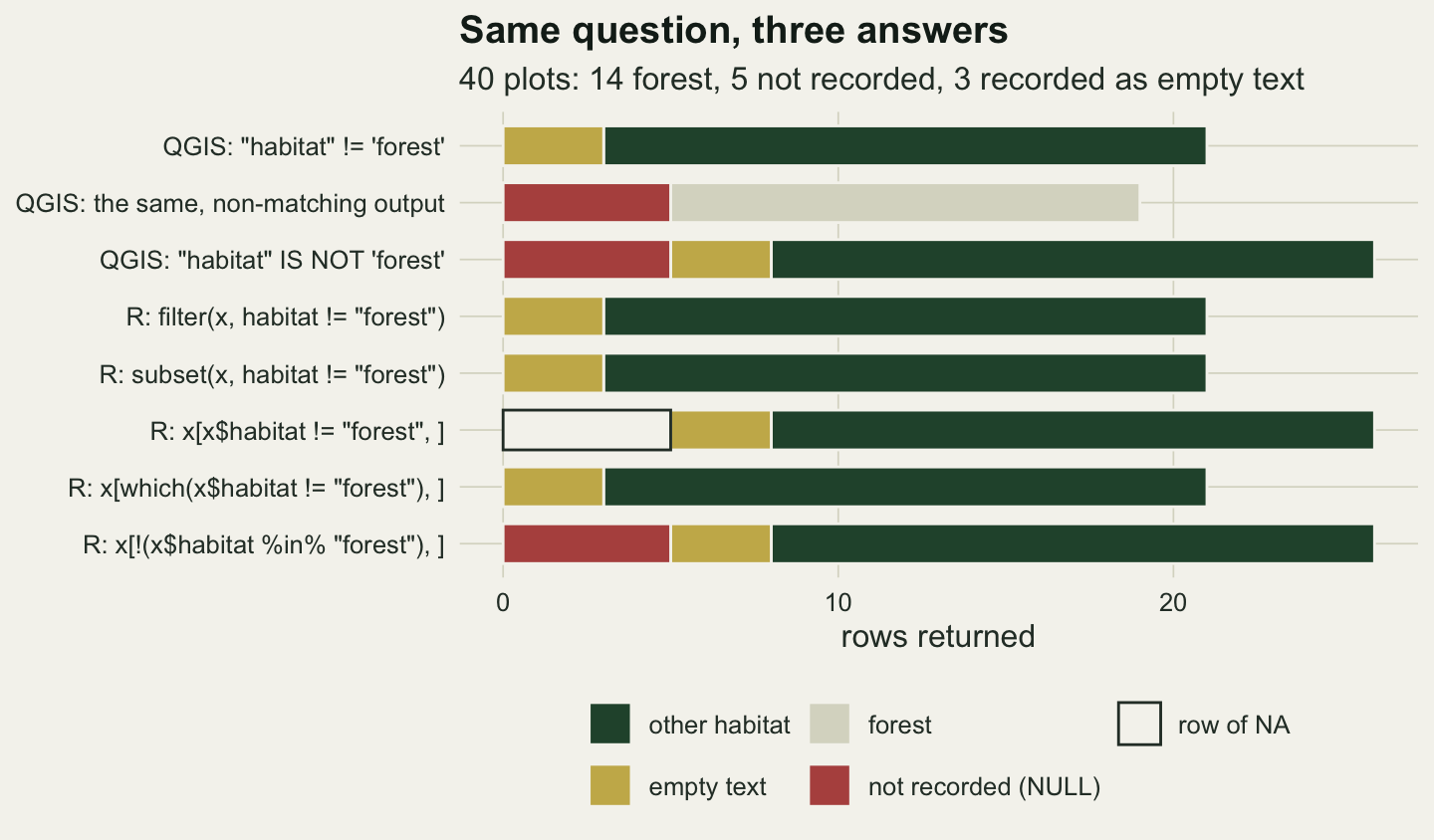
What the export keeps
The last step of the handoff is the file. In the desktop it is a right click on the layer, Export > Save Features As, with the format set to GeoPackage or to Comma Separated Value; the CSV writer’s options, including STRING_QUOTING, sit under Layer Options in the same dialog. The third call below asks for every string to be quoted, which is the natural thing to try if the problem is that an empty string and a missing value both look like nothing.
qgis_process run native:savefeatures -- INPUT=survey-plots.gpkg OUTPUT=survey-export.gpkg
qgis_process run native:savefeatures -- INPUT=survey-plots.gpkg OUTPUT=survey-export.csv
qgis_process run native:savefeatures -- INPUT=survey-plots.gpkg OUTPUT=survey-quoted.csv \
  LAYER_OPTIONS=STRING_QUOTING=ALWAYS
QGIS can also read that CSV back, in two ways. Layer > Add Layer > Add Delimited Text Layer (Ctrl+Shift+T) uses the delimited text provider; Layer > Add Layer > Add Vector Layer (Ctrl+Shift+V) opens the same file through GDAL, the OGR provider. The script below first runs the selection promised in the filter section, then opens both CSV files both ways and counts NULL and empty text. It was run headless with the Python that ships with QGIS (/usr/bin/python3.12 here, after the export line of the first block); setPrefixPath("/usr") is the Linux install location. In the desktop, open Plugins > Python Console (Ctrl+Alt+P), click Show Editor, paste the script without the four lines that set up, start and stop app, add an os.chdir() to the post folder below the imports, and press Run Script; pasted line by line at the console prompt, the blocks do not parse.
import csv, os
from qgis.core import QgsApplication, QgsVectorLayer, QgsFeatureRequest
from qgis.PyQt.QtCore import QUrl
QgsApplication.setPrefixPath("/usr", True)
app = QgsApplication([], False)
app.initQgis()
survey = QgsVectorLayer(os.path.abspath("survey-plots.gpkg"), "survey", "ogr")
with open("qgis-select.csv", "w", newline="") as out:
    writer = csv.writer(out)
    writer.writerow(["test", "selected"])
    for key, expr in [("ne_forest", "\"habitat\" != 'forest'"),
                      ("isnot_forest", "\"habitat\" IS NOT 'forest'")]:
        survey.selectByExpression(expr)
        writer.writerow([key, survey.selectedFeatureCount()])
tests = {"habitat_null": '"habitat" IS NULL',
         "habitat_blank": "\"habitat\" = ''",
         "cover_null": '"cover" IS NULL'}
rows = []
for fname in ["survey-export.csv", "survey-quoted.csv"]:
    path = os.path.abspath(fname)
    dt_uri = QUrl.fromLocalFile(path).toString() + "?delimiter=,&geomType=none"
    for provider, source in [("ogr", path), ("delimitedtext", dt_uri)]:
        layer = QgsVectorLayer(source, "readback", provider)
        row = {"file": fname, "provider": provider,
               "cover_type": layer.fields().field("cover").typeName()}
        for key, expr in tests.items():
            request = QgsFeatureRequest().setFilterExpression(expr)
            row[key] = sum(1 for _ in layer.getFeatures(request))
        rows.append(row)
with open("qgis-csv-readback.csv", "w", newline="") as out:
    writer = csv.DictWriter(out, fieldnames=list(rows[0]))
    writer.writeheader()
    writer.writerows(rows)
del survey, layer  # release the layers first, or the headless run crashes on exit
app.exitQgis()
third_field <- function(lines) sub("^[^,]*,[^,]*,([^,]*),.*$", "\\1", lines[-1])
raw_plain <- third_field(readLines("survey-export.csv"))
raw_quoted <- third_field(readLines("survey-quoted.csv"))
null_ids <- which(is.na(survey$habitat)); blank_ids <- which(survey$habitat %in% "")
text_null <- unique(raw_plain[null_ids]); text_blank <- unique(raw_plain[blank_ids])
qtext_null <- unique(raw_quoted[null_ids]); qtext_blank <- unique(raw_quoted[blank_ids])
csv_cols <- names(read.csv("survey-export.csv"))
state_of <- function(v) c(missing = sum(is.na(v)), empty = sum(v %in% ""),
value = sum(!is.na(v) & !(v %in% "")))
from_counts <- function(n_missing, n_empty) c(missing = n_missing, empty = n_empty,
value = n_plot - n_missing - n_empty)
back <- read.csv("qgis-csv-readback.csv")
b_ogr <- back[back$file == "survey-export.csv" & back$provider == "ogr", ]
b_dt <- back[back$file == "survey-export.csv" & back$provider == "delimitedtext", ]
count_cols <- c("habitat_null", "habitat_blank", "cover_null")
same_quoted <- all(back[back$file == "survey-quoted.csv", count_cols] ==
back[back$file == "survey-export.csv", count_cols])
gp_back <- st_read("survey-export.gpkg", quiet = TRUE)
rc_plain <- read.csv("survey-export.csv")
rc_nastr <- read.csv("survey-export.csv", na.strings = "")
st_csv <- st_read("survey-export.csv", quiet = TRUE)
routes <- rbind( # row names are markdown code spans for the table; the figure drops the backticks
"QGIS, as stored in the GeoPackage" = from_counts(n_q_null, n_q_blank),
"GeoPackage, read by `st_read()`" = state_of(gp_back$habitat),
"CSV, read by `read.csv()`" = state_of(rc_plain$habitat),
"CSV, `read.csv(na.strings = \"\")`" = state_of(rc_nastr$habitat),
"CSV, read by `st_read()`" = state_of(st_csv$habitat),
"CSV, QGIS OGR provider" = from_counts(b_ogr$habitat_null, b_ogr$habitat_blank),
"CSV, QGIS delimited text provider" = from_counts(b_dt$habitat_null, b_dt$habitat_blank))
knitr::kable(routes, caption = "The forty habitat values after each route out of QGIS and back in.")| missing | empty | value | |
|---|---|---|---|
| QGIS, as stored in the GeoPackage | 5 | 3 | 32 |
GeoPackage, read by st_read() |
5 | 3 | 32 |
CSV, read by read.csv() |
0 | 8 | 32 |
CSV, read.csv(na.strings = "") |
8 | 0 | 32 |
CSV, read by st_read() |
0 | 8 | 32 |
| CSV, QGIS OGR provider | 0 | 8 | 32 |
| CSV, QGIS delimited text provider | 8 | 0 | 32 |
cover_na <- c(gpkg = sum(is.na(gp_back$cover)), read_csv = sum(is.na(rc_plain$cover)),
              st_read_csv = sum(is.na(st_csv$cover)), st_read_empty = sum(st_csv$cover %in% ""),
              ogr = b_ogr$cover_null, delim = b_dt$cover_null)
cover_class <- c(read_csv = class(rc_plain$cover), st_read_csv = class(st_csv$cover))
n_gap_csv <- sum(raw_plain == "")
The plain CSV writes both kinds of gap the same way. The habitat field of the unrecorded plots reads '' in the file, and the habitat field of the plots recorded as empty text reads '': nothing between two commas, in all 8 rows. Quoting every string does not help, because the writer quotes the NULL as well; in the quoted file both groups read "" and "". Once the file exists, no reader can separate them, and every reader in the table above picks one of the two answers for all 8. The file also gained a column and lost one: its columns are fid, plot_id, habitat, cover, the first being the GeoPackage feature id and the geometry gone, since no geometry option was set.
read.csv() calls all 8 gaps empty text, which is the text column rule from the reading field data post, and the 5 plots nobody visited now pass a habitat != "forest" filter as if someone had recorded them. The usual repair, na.strings = "", turns all 8 into NA, so the 3 plots that were recorded as empty become unrecorded. It swaps one error for the other; it does not undo either. st_read() on the CSV goes through GDAL, whose CSV reader treats an empty field as an empty string unless told otherwise (its EMPTY_STRING_AS_NULL open option is off by default), so it agrees with read.csv(). QGIS disagrees with itself: the OGR provider reads 8 empty strings and 0 NULL, the delimited text provider reads 8 NULL and 0 empty strings. The quoted file gave each provider exactly the counts the plain file gave it (TRUE).
The numeric column does less damage but is not tidy either. read.csv() reads the cover column as integer with 6 NA, the number removed, and the delimited text provider finds the same 6 NULL. st_read() and the OGR provider read every column of a CSV as text unless told to guess types, so there cover arrives as character with 6 empty strings and 0 NULL in QGIS. The GeoPackage route keeps everything: 5 missing, 3 empty and 6 missing cover values, as stored. A GeoPackage is an SQLite database, and a SQL NULL is a value of its own there, not a way of writing text.
Writing NULL down as a code
If a CSV is required anyway, by a repository or a collaborator, make the missing value something the file can hold before it is written. coalesce() does that in one field calculator call: given the name of an existing field, the algorithm replaces that field in its output.
qgis_process run native:fieldcalculator -- INPUT=survey-plots.gpkg FIELD_NAME=habitat \
  FIELD_TYPE=2 FORMULA="coalesce(\"habitat\", 'NR')" OUTPUT=survey-coded.csv
coded <- read.csv("survey-coded.csv", na.strings = "NR")
coded_state <- state_of(coded$habitat)
coded_cols <- identical(names(coded), csv_cols)
coded_same <- identical(which(is.na(coded$habitat)), null_ids) &&
identical(which(coded$habitat %in% ""), blank_ids)Read back with na.strings = "NR", the file gives 5 missing habitats and 3 empty ones, on the same plots as the original (TRUE), and the file has the same columns as the plain export (TRUE), so no second habitat field was added. The code has to be one that cannot occur as a real value, and it has to be written down next to the file, because nothing in a CSV says what NR means.
routes_all <- rbind(routes, "coded CSV, read.csv(na.strings = \"NR\")" = coded_state)
route_names <- gsub("`", "", rownames(routes_all))
route_long <- data.frame(route = factor(rep(route_names, 3), levels = rev(route_names)),
                         state = rep(c("missing", "empty text", "a habitat class"), each = length(route_names)),
                         plots = c(routes_all[, "missing"], routes_all[, "empty"], routes_all[, "value"]))
route_long$state <- factor(route_long$state, levels = c("a habitat class", "empty text", "missing"))
ggplot(route_long, aes(plots, route, fill = state)) +
  geom_col(width = 0.7, colour = te_paper, linewidth = 0.3) +
  scale_fill_manual(values = c("a habitat class" = te_forest, "empty text" = te_gold,
                               "missing" = te_rust), name = NULL) +
  labs(x = "plots", y = NULL, title = "Two routes keep NULL and empty text apart",
       subtitle = sprintf("%d plots not recorded, %d recorded as empty text", n_null, n_blank)) +
  theme_datasheet() + theme(legend.position = "bottom", plot.title.position = "plot")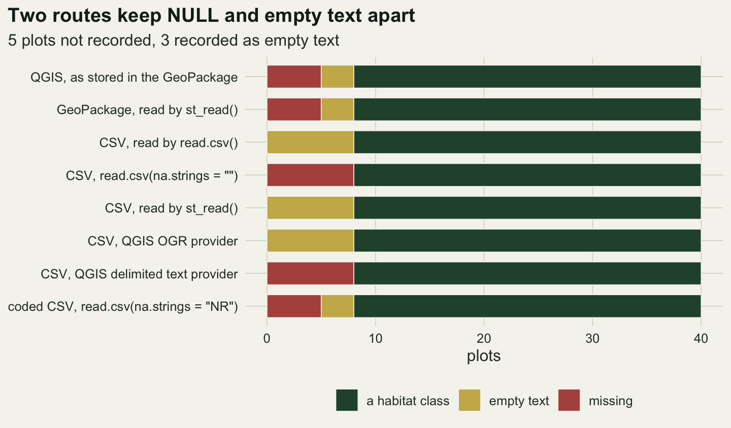
What to do about it
Move layers between QGIS and R as GeoPackage. It keeps NULL, empty text and the column types, and st_read() returns them as NA, "" and the right classes. Use a CSV only as an export, after writing the missing values of text columns as a code with coalesce(), and read it back with that code in na.strings; numeric blanks already come back from read.csv() as NA.
In QGIS, decide what a filter should do with NULL before running it. "habitat" != 'forest' quietly files the unrecorded plots with the forest ones. "habitat" IS NOT 'forest' keeps them, and coalesce("habitat", 'not recorded') != 'forest' keeps them under a name you can count. When a QGIS aggregate goes into a report, remember that mean() and count() have already dropped the NULL rows, and count_missing() gives the number they dropped.
In R, check the gaps with table(x$habitat, useNA = "ifany") against the QGIS attribute table before filtering. Filter with filter(), subset() or which() rather than a bare logical index, or write is.na() into the condition. Pass na.rm = TRUE knowingly, not by habit, and never build labels with paste0() from a column that can hold NA.
What to report: how missing values were coded in the file that was analysed, how many records were missing in each attribute, and how each filter treated them. “5 plots with no habitat recorded were kept as a separate class” is a sentence a reader can check; “non-forest plots (n = 21)” is not, because the reader cannot tell whether the unrecorded plots were in it.
Honest limits
Every QGIS result here comes from one build, 3.34.4 on Linux with GDAL 3.8.4 underneath. The expression rules shown match the QGIS 3.40 manual, but the CSV behaviour is GDAL’s and the delimited text provider’s, and either can change between versions; rerun the commands on your own installation before relying on the counts. The field calculator measured is the Processing algorithm. The attribute table’s Field Calculator uses the same expression engine, but it writes into the layer being edited, and that path was not run. The PyQGIS check of Select Features by Expression compared counts, not the plots selected.
The R side covers base R, dplyr and sf. Other readers, such as readr or data.table, have their own rules for empty fields and were not tested, and neither was a shapefile, whose attribute file is the subject of the shapefile post. Everything is synthetic, and in real data the two kinds of gap are rarely labelled as cleanly as here: often nobody knows whether an empty cell meant “not recorded” or “nothing to record”. The point is narrower. Whatever the difference was, a GeoPackage keeps it, a plain CSV throws it away, and a filter that does not mention NULL makes a decision about those plots on your behalf.
References
Pebesma E 2018 The R Journal 10(1):439-446 (10.32614/RJ-2018-009)
QGIS Development Team 2024 QGIS User Guide 3.40: Expressions, list of functions and operators (https://docs.qgis.org/3.40/en/docs/user_manual/expressions/functions_list.html)
GDAL contributors 2024 GDAL 3.8.4 documentation source: CSV driver (https://github.com/OSGeo/gdal/blob/v3.8.4/doc/source/drivers/vector/csv.rst)
Open Geospatial Consortium 2021 OGC GeoPackage Encoding Standard 1.3.1, OGC 12-128r18 (https://www.geopackage.org/spec131/)