---
title: "What a shapefile loses: names, times and types"
description: "A shapefile round trip returns the geometry exactly and then rewrites the attribute table: names abbreviated, the clock dropped, logicals made integer."
date: "2026-08-12 11:00"
categories: [R, sf, spatial, data management, ecology tutorial]
image: thumbnail.png
image-alt: "Two twenty-four hour clock faces of visit times, one with the points occupying the morning and early afternoon arc and the other with the points in a single radial line at midnight."
date-modified: "2026-10-14"
---
*Corrected 14 October 2026: the post said the GDAL warning about the date field is invisible in a Quarto document; it is printed unless the chunk hides warnings, as the write chunk here does. It also named summing the integer that replaces the logical as a hazard, which it is not, and said the GeoPackage loses only the factor; `sf` also reads its date-times back without a time zone, so in a session set to another zone the clock hours print shifted.*
*Corrected 7 October 2026: the post said `sf` abbreviates each long field name until it fits and that a missing column drops out of a `data.frame()` call; it now says that once any name is too long every name is passed to `abbreviate()` with a target shorter than the limit, and that `data.frame()` stops with an error. The closing limits no longer say that an evenly spread schedule loses no information, or that the cap on the number of fields never stops the write.*
*Corrected 30 September 2026: the post said `sf` strips vowels and repeated letters from long field names; it now says the names go through base R's `abbreviate()`, which drops lower-case vowels and then lower-case consonants from the right.*
*Corrected 27 September 2026: the closing limits said the shapefile format has no way to store a null geometry; it does have a null shape type, so that item has been removed.*
The geometry is the part everyone worries about, and the geometry is the part that survives. Write a set of plot locations to a shapefile, read them back, and the coordinates are identical to the last bit and the coordinate reference system comes back intact. What changes is the table sitting beside the points, and it changes without an error.
This is the spatial twin of a problem that also afflicts plain text: the values return, the decisions you put on top of them do not. A shapefile is worse than a CSV in one specific way, though. A CSV at least gives you back the column name you wrote.
## An attribute table an ecologist would actually build
Twenty-four vegetation plots, a browse index measured in two seasons, an ordered cover class, the time each plot was visited, a logical for whether browsing was seen at all, and a soil pH with two missing values.
```{r setup}
#| message: false
#| warning: false
library(sf)
library(ggplot2)

te_paper  <- "#f5f4ee"
te_ink    <- "#16241d"
te_body   <- "#2c3a31"
te_forest <- "#275139"
te_rust   <- "#b5534e"
te_gold   <- "#c9b458"
te_line   <- "#dad9ca"

theme_datasheet <- function() {
  theme_minimal(base_size = 12) +
    theme(plot.background  = element_rect(fill = te_paper, colour = NA),
          panel.background = element_rect(fill = te_paper, colour = NA),
          panel.grid.major = element_line(colour = te_line, linewidth = 0.3),
          panel.grid.minor = element_blank(),
          text             = element_text(colour = te_body),
          plot.title       = element_text(colour = te_ink, face = "bold"),
          axis.text        = element_text(colour = te_body))
}

set.seed(20260812)
n <- 24

# the plots were visited during the working day, centred on mid-morning
hours <- (11 + rnorm(n, 0, 2.1)) %% 24

field <- data.frame(
  site_code           = sprintf("S%02d", seq_len(n)),
  browse_index_spring = round(runif(n, 0, 1), 3),
  browse_index_autumn = round(runif(n, 0, 1), 3),
  canopy_cover_class  = factor(sample(c("low", "medium", "high"), n, TRUE),
                               levels = c("low", "medium", "high"),
                               ordered = TRUE),
  visit_time          = as.POSIXct("2026-05-01", tz = "UTC") + 3600 * hours,
  browsed             = sample(c(TRUE, FALSE), n, TRUE),
  soil_ph             = round(runif(n, 4.2, 7.8), 2),
  stringsAsFactors    = FALSE)
field$soil_ph[c(4, 17)] <- NA

plots <- st_as_sf(cbind(field,
                        x = 400000 + runif(n, 0, 8000),
                        y = 5050000 + runif(n, 0, 8000)),
                  coords = c("x", "y"), crs = 32634)
str(field$canopy_cover_class)
```
Now deposit it twice: once as a shapefile, because that is still what most repositories and most collaborators ask for, and once as a GeoPackage, so there is something to compare against.
```{r write}
#| warning: false
dir_out <- file.path(tempdir(), "deposit")
dir.create(dir_out, showWarnings = FALSE)
shp  <- file.path(dir_out, "plots.shp")
gpkg <- file.path(dir_out, "plots.gpkg")

st_write(plots, shp,  quiet = TRUE, delete_dsn = TRUE)
st_write(plots, gpkg, quiet = TRUE, delete_dsn = TRUE)

from_shp  <- st_read(shp,  quiet = TRUE)
from_gpkg <- st_read(gpkg, quiet = TRUE)
```
## The geometry is exact and the names are not
First the good news, and check it strictly: `identical` rather than `all.equal`, because the claim is that nothing moved at all, and `all.equal` would pass a shift of several millimetres on coordinates this large.
```{r geometry}
c(coordinates = identical(st_coordinates(plots), st_coordinates(from_shp)),
  crs         = st_crs(plots) == st_crs(from_shp))
```
Nothing moved. Now the column names.
```{r names}
nm <- setdiff(names(from_shp), "geometry")
data.frame(deposited = setdiff(names(plots), "geometry"), shapefile = nm)
```
The DBF file that carries a shapefile's attributes allows ten characters per field name, so something has to give, and `sf` abbreviates rather than truncates: once any name is over the limit, it passes every name to base R's `abbreviate()` with a minimum length below the limit, which drops lower-case vowels and then lower-case consonants, working from the right, until each name is down to that minimum, and keeps a name longer only where that is needed to keep the names distinct. So `site_code` and `visit_time` were renamed although they fit the limit, `soil_ph` and `browsed` were short enough to survive, and `canopy_cover_class` came back as **`r nm[4]`**, which is guessable. The pair that matters is the browse index.
```{r seasons}
nm[2:3]
```
Spring and autumn have been reduced to a trailing **`r substr(nm[2], 10, 10)`** and a trailing **`r substr(nm[3], 10, 10)`**. The two columns are still there, still in the right order, still holding the right numbers. What is gone is the only thing in the file that said which one was which, and the surviving letters do not say it either: the `t` is the third letter of autumn, so alphabetical intuition points the wrong way if anyone reaches for it.
The immediate practical consequence is that code written against the deposited object stops finding its columns, and `$` does not complain.
```{r dollar}
c(spring_column_found = !is.null(from_shp$browse_index_spring),
  time_column_found   = !is.null(from_shp$visit_time))
```
`NULL` is not an error. It flows into `mean()` as `NA` and into an arithmetic expression as a zero-length vector, and each of those failures happens somewhere other than the line that caused it. A `data.frame()` call with other columns does stop, but with a complaint about differing numbers of rows that does not name the missing column.
## The clock is gone
The DBF format has a date type and no date-time type. A `POSIXct` column is therefore written as a date, and GDAL says so at write time, in a warning that scrolls past in a script and does not appear in a Quarto document whose chunk sets `warning: false`, as the write chunk above does.
```{r classes}
cls <- function(z) sapply(st_drop_geometry(z), function(v) class(v)[1])
data.frame(column     = names(cls(plots)),
           deposited  = unname(cls(plots)),
           shapefile  = unname(cls(from_shp)),
           geopackage = unname(cls(from_gpkg)))
```
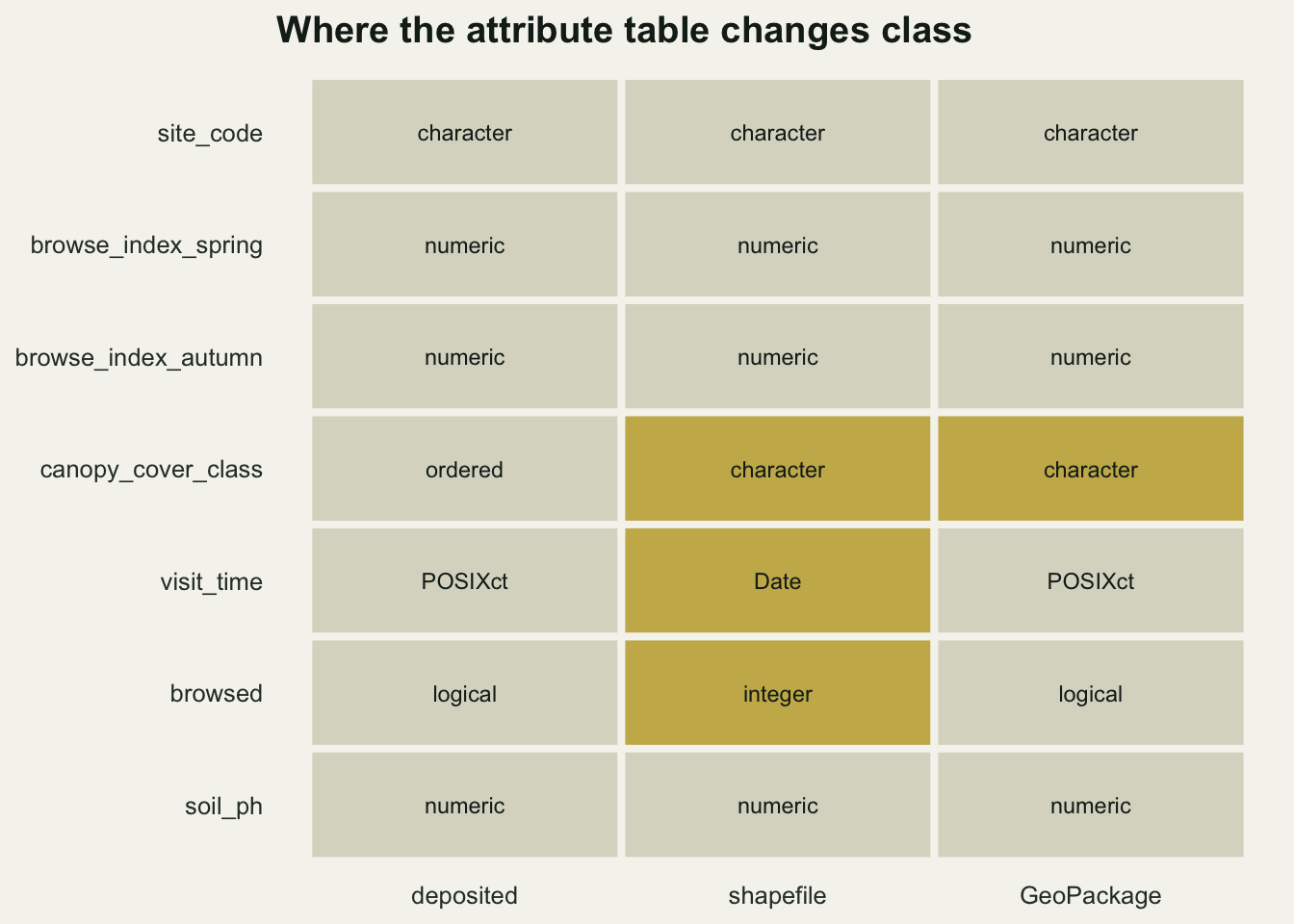
Three rows changed. The ordered factor became character, which loses the level ordering exactly as a CSV does. The logical became an integer, which is harmless for sums and means but not for code that compares it with text: a filter on `browsed == "TRUE"` gets nothing back. The third is the expensive one.
```{r clock}
recovered <- st_drop_geometry(from_shp)[[5]]
c(class = class(recovered)[1], distinct_values = length(unique(recovered)))
```
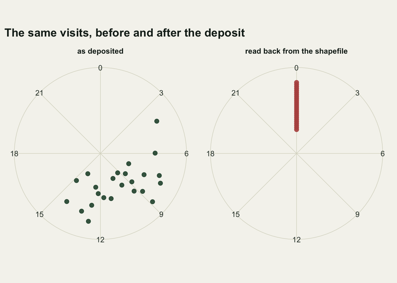
Every visit now happened at midnight on the same day. If those timestamps were camera trap detections, or acoustic triggers, or anything else whose analysis is a distribution over the twenty-four hour cycle, the analysis is no longer possible from the deposited file. Here is what that costs, in the three numbers such a study reports.
```{r activity}
circ_mean <- function(h) {
  a <- 2 * pi * h / 24
  (atan2(mean(sin(a)), mean(cos(a))) %% (2 * pi)) * 24 / (2 * pi)
}
circ_r <- function(h) {
  a <- 2 * pi * h / 24
  sqrt(mean(sin(a))^2 + mean(cos(a))^2)
}
night <- function(h) mean(h < 6 | h >= 18)

after_h <- rep(0, n)   # midnight, for every record
round(c(mean_hour_before = circ_mean(hours),
        mean_hour_after  = circ_mean(after_h),
        r_before         = circ_r(hours),
        r_after          = circ_r(after_h),
        night_before     = night(hours),
        night_after      = night(after_h)), 3)
```
The mean hour moves from `r sprintf("%.1f", circ_mean(hours))` to `r sprintf("%.1f", circ_mean(after_h))`, and the mean vector length, which measures how tightly the records cluster on the circle, rises from `r sprintf("%.3f", circ_r(hours))` to `r sprintf("%.3f", circ_r(after_h))`: one is the value for records concentrated in a few hours of the day, the other is the value for records at a single instant. The share that a daylight and darkness split would call nocturnal moves from `r sprintf("%.2f", night(hours))` to `r sprintf("%.2f", night(after_h))`. Nothing warns about any of this. A total collapse like this one is at least conspicuous: a mean vector length of exactly 1 is not a result anyone would publish without looking. The dangerous version is partial, where one deposited file in a series lost its clock and the others did not, and the pooled distribution simply grows a spike at midnight.
```{r fig-clock}
#| fig-cap: "Visit times on a twenty-four hour clock face, as deposited and as read back from the shapefile. The distance from the centre only separates points that would otherwise overlap."
#| fig-alt: "Two circular panels with hour labels around the rim and hours running clockwise from zero at the top. In the left panel the twenty-four points occupy just under half the rim, from the early morning hours round to the early afternoon, at scattered distances from the centre. In the right panel the twenty-four points form a single straight radial line at the zero mark."
clock <- rbind(
  data.frame(hour = hours,   panel = "as deposited"),
  data.frame(hour = after_h, panel = "read back from the shapefile"))
clock$panel <- factor(clock$panel, levels = unique(clock$panel))
# the radius separates overlapping points and carries no information
clock$rad   <- ave(seq_len(nrow(clock)), clock$panel, FUN = seq_along)

ggplot(clock, aes(x = hour, y = 0.32 + 0.03 * rad)) +
  geom_point(aes(colour = panel), size = 2.2, alpha = 0.9) +
  facet_wrap(~ panel) +
  coord_polar(theta = "x", start = 0) +
  scale_x_continuous(limits = c(0, 24), breaks = seq(0, 21, 3)) +
  scale_y_continuous(limits = c(0, 1.12), breaks = NULL) +
  scale_colour_manual(values = c(te_forest, te_rust)) +
  labs(x = NULL, y = NULL,
       title = "The same visits, before and after the deposit") +
  theme_datasheet() +
  theme(legend.position = "none",
        panel.grid.major = element_line(colour = te_line, linewidth = 0.3),
        strip.text = element_text(colour = te_ink, face = "bold"))
```
## What survives, column by column
Missing values are the case worth checking rather than assuming, because the folklore says a shapefile turns `NA` into zero.
```{r missing}
c(na_deposited = sum(is.na(field$soil_ph)),
  na_shapefile = sum(is.na(from_shp$soil_ph)),
  na_geopackage = sum(is.na(from_gpkg$soil_ph)))
```
They come back. A blank numeric field in the DBF is read as `NA`, and has been for many GDAL versions. The folklore comes from software that writes a fill value such as `-9999` or `0` on the way out, which is a choice made by the exporting program and not a property of the format. Worth knowing which of those your GIS does before you blame the file.
```{r fig-types}
#| fig-cap: "Class of each attribute column as deposited and as recovered from each format."
#| fig-alt: "A grid of cells with the seven attribute columns down the side and three format labels along the bottom, each cell giving an R class. Three cells are highlighted in the shapefile column, for the ordered factor, the date-time and the logical, and one in the GeoPackage column, for the ordered factor."
tab <- data.frame(
  column = rep(names(cls(plots)), 3),
  format = rep(c("deposited", "shapefile", "GeoPackage"), each = 7),
  class  = c(unname(cls(plots)), unname(cls(from_shp)), unname(cls(from_gpkg))))
tab$format <- factor(tab$format,
                     levels = c("deposited", "shapefile", "GeoPackage"))
tab$column <- factor(tab$column, levels = rev(names(cls(plots))))
tab$changed <- tab$class != rep(unname(cls(plots)), 3)

ggplot(tab, aes(x = format, y = column)) +
  geom_tile(aes(fill = changed), colour = te_paper, linewidth = 1.4) +
  geom_text(aes(label = class), size = 3.1, colour = te_ink) +
  scale_fill_manual(values = c(`FALSE` = te_line, `TRUE` = te_gold)) +
  labs(x = NULL, y = NULL,
       title = "Where the attribute table changes class") +
  theme_datasheet() +
  theme(legend.position = "none",
        panel.grid.major = element_blank())
```
The GeoPackage column is the control. It is a SQLite database with a real type system, so the visit times, the logical and the long field names all come back. It loses the factor, as the shapefile does, and that is not a format failure: no file format on that list stores an R factor, because the level ordering is a statement about the analysis and not about the data. The time zone goes too, more quietly: the file holds the visit times in UTC, but `sf` reads them back as a `POSIXct` column without a time zone attribute, so in a session set to any other zone the clock hours print shifted by the offset unless the zone is set again.
## Depositing so the table survives
Three things, in order of how much they buy you.
Use GeoPackage as the working format. A single file, no sidecar files to lose, no ten character limit, real types, and every GIS made in the last decade opens it. If a collaborator or a repository insists on a shapefile, write the shapefile as well and treat it as the export it is, not as the archive.
Keep the ordering out of the file. A small dictionary that names the columns, their types, their units and the level set in order is readable by a person and by a script, and it is the only place the ordering can live.
```{r dictionary}
dictionary <- data.frame(
  column = c("canopy_cover_class", "visit_time", "browsed"),
  type   = c("ordered factor", "POSIXct, UTC", "logical"),
  detail = c(paste(levels(field$canopy_cover_class), collapse = " < "),
             "time of day is the analysis variable",
             "TRUE means browsing seen"))
dictionary
```
Then rebuild from the dictionary rather than from whatever the file happens to return, and check the rebuild by re-running the analysis on it. If a number moves, the deposit is not the analysis.
```{r rebuild}
lv <- strsplit(dictionary$detail[1], " < ")[[1]]
rebuilt <- from_gpkg
rebuilt$canopy_cover_class <- factor(rebuilt$canopy_cover_class,
                                     levels = lv, ordered = TRUE)

c(levels_from_gpkg = paste(levels(factor(from_gpkg$canopy_cover_class)),
                           collapse = " < "),
  levels_rebuilt   = paste(levels(rebuilt$canopy_cover_class), collapse = " < "))
```
## Honest limits
The abbreviation shown here is `sf`'s, not the shapefile's. Write the same object from QGIS and you get plain truncation to ten characters instead, which collides where `sf` does not: two columns whose first ten characters agree end up as one name plus a numbered variant. Either way the season labels are gone; the two tools lose them differently.
Nothing above depends on the values being synthetic. What changes with real data is how much information the three activity summaries carried in the first place, not what the file returns: every record comes back at midnight whatever its schedule. A schedule that was already spread evenly round the clock would be no exception: its mean vector length would jump from near zero to one, and a file that showed no daily rhythm would now show a single spike at midnight. Only records that were all taken at midnight already would come through unchanged.
The date itself survives, so a study whose time variable is the day rather than the hour is unaffected. So is any analysis that reads its attributes from the original object and uses the shapefile only to draw a map. The loss is real when the deposited file is the thing someone reanalyses, which is exactly the situation archiving is for.
Finally, the field name limit is not the only shapefile limit, only the one that shows up first. Character fields are cut at 254 characters without stopping the write, and the number of fields is capped too: GDAL only warns once a layer has more fields than some DBF readers support, but stops the write at the hard limit the DBF header sets.
## References
Pebesma E 2018 The R Journal 10(1):439-446 (10.32614/RJ-2018-009)
Bivand RS 2021 Journal of Geographical Systems 23(4):515-546 (10.1007/s10109-020-00336-0)
Wilkinson MD, Dumontier M, Aalbersberg IJ, et al 2016 Scientific Data 3:160018 (10.1038/sdata.2016.18)
## Related tutorials
- [What a CSV loses: archiving an R analysis](../what-a-csv-loses/)
- [Checking a vector layer before you measure](../checking-a-vector-layer/)
- [Running QGIS from the command line](../running-qgis-from-the-command-line/)
- [QGIS NULL and R NA: what survives the trip](../qgis-null-and-r-na/)