library(ggplot2)

te_pal <- list(forest = "#275139", green = "#2f8f63", sage = "#93a87f",
               clay = "#b5534e", gold = "#cda23f", line = "#dad9ca",
               ink = "#16241d", paper = "#f5f4ee")

theme_te <- function() {
  theme_minimal(base_size = 12) +
    theme(panel.grid.minor = element_blank(),
          panel.grid.major = element_line(colour = "#e7e6dc"),
          plot.background = element_rect(fill = "#f5f4ee", colour = NA),
          panel.background = element_rect(fill = "#f5f4ee", colour = NA),
          plot.title = element_text(face = "bold", colour = te_pal$ink),
          axis.title = element_text(colour = "#2c3a31"))
}Dates and times in ecological data
R
data cleaning
ecology tutorial
ggplot2
Parsing field dates in base R: where as.Date returns a silent NA, what a swapped day and month does to a flight period, and how summer time bends activity data.
Step 5 of the Tidy Ecology course, Part one: get the data into R.
A colleague sends you the season’s first-flowering records as one spreadsheet export. It has been assembled from three sources: the national recording scheme, a partner network that took over the lowland sites this year, and a volunteer group. The date column looks fine. You read it, you compute a mean flowering date, you compare it with last year, and the answer is that flowering ran six days later than in 2018. You write that down.
Nothing in the script failed. Nothing printed a warning. The number is of the right size, the right sign is plausible for a cool spring, and the only reason to doubt it is that the three sources did not write their dates the same way, and R quietly discarded the ones it could not read.
This post is about that class of failure, and it is a narrow post on purpose: it is about parsing and about arithmetic. What a date means once you have it, how day of year behaves at the year boundary and in a leap year, and how to summarise event timing are all in phenology in R: day of year and event timing. Here the question is earlier and duller: did the calendar value in memory come from the text in the file, and does subtracting one from another give the number of days you think it does.
Four measurements follow. Every simulation is a working ecological analysis run twice, once with the date handling wrong and once with it right, and the number that matters each time is the change in the ecological answer rather than the number of broken rows.
When as.Date gives up without saying so
The study is a first-flowering survey along an elevation gradient, 180 permanent sites between 200 and 1400 metres, recorded in 2018 and again in 2019. Flowering is later higher up, at three days per hundred metres, and the simulated 2019 season is set a little earlier than 2018. In 2018 one scheme recorded everything and wrote its dates in the ISO order, year first. In 2019 the sites below 700 metres were handed over: the middle band to a partner network that writes slashes with the day first, the lowest sites to a volunteer group that writes dots and a two-digit year.
That is the whole setup. The sites are identical between years, the elevations are identical, and the only thing that changed is who typed the date.
set.seed(20260818)
n_site <- 180
elev <- round(runif(n_site, 200, 1400))
doy_2018 <- round(96.0 + 3.0 * (elev - 200) / 100 + rnorm(n_site, 0, 4.2))
doy_2019 <- round(94.8 + 3.0 * (elev - 200) / 100 + rnorm(n_site, 0, 4.2))
d_2018 <- as.Date("2018-01-01") + doy_2018 - 1
d_2019 <- as.Date("2019-01-01") + doy_2019 - 1

source_2019 <- ifelse(elev >= 700, "scheme",
               ifelse(elev >= 450, "partner", "volunteers"))
written_2018 <- format(d_2018, "%Y-%m-%d")
written_2019 <- ifelse(source_2019 == "scheme", format(d_2019, "%Y-%m-%d"),
                ifelse(source_2019 == "partner", format(d_2019, "%d/%m/%Y"),
                       format(d_2019, "%d.%m.%y")))
print(table(source_2019))
source_2019
partner scheme volunteers
44 102 34 print(head(data.frame(elevation = elev, source = source_2019,
written = written_2019), 6)) elevation source written
1 212 volunteers 09.04.19
2 550 partner 12/04/2019
3 423 volunteers 12.04.19
4 932 scheme 2019-04-17
5 458 partner 05/04/2019
6 1261 scheme 2019-05-09The analysis script does what almost every analysis script does. It names the format it expects and moves on.
read_2018 <- as.Date(written_2018, format = "%Y-%m-%d")
read_2019 <- as.Date(written_2019, format = "%Y-%m-%d")
got_2018 <- as.numeric(format(read_2018, "%j"))
got_2019 <- as.numeric(format(read_2019, "%j"))

q10 <- function(x) as.numeric(quantile(x, 0.10, na.rm = TRUE, names = FALSE))
q90 <- function(x) as.numeric(quantile(x, 0.90, na.rm = TRUE, names = FALSE))
true_change <- mean(doy_2019) - mean(doy_2018)
naive_change <- mean(got_2019, na.rm = TRUE) - mean(got_2018, na.rm = TRUE)
f_true <- lm(doy_2019 ~ I(elev / 100))
f_kept <- lm(got_2019 ~ I(elev / 100))

round(c(sites = n_site,
        rows_lost = sum(is.na(read_2019)),
        rows_lost_percent = 100 * mean(is.na(read_2019)),
        highest_lost_site_metres = max(elev[is.na(read_2019)]),
        mean_elevation_kept = mean(elev[!is.na(read_2019)]),
        mean_elevation_lost = mean(elev[is.na(read_2019)]),
        true_mean_doy_2018 = mean(doy_2018),
        true_mean_doy_2019 = mean(doy_2019),
        true_change_days = true_change,
        reported_mean_doy_2019 = mean(got_2019, na.rm = TRUE),
        reported_change_days = naive_change,
        error_days = naive_change - true_change,
        true_start_of_season = q10(doy_2019),
        reported_start_of_season = q10(got_2019),
        start_shift_days = q10(got_2019) - q10(doy_2019),
        true_season_span = q90(doy_2019) - q10(doy_2019),
        reported_season_span = q90(got_2019) - q10(got_2019),
        true_slope_days_per_100m = coef(f_true)[2],
        kept_slope_days_per_100m = coef(f_kept)[2],
        true_slope_se = summary(f_true)$coefficients[2, 2],
        kept_slope_se = summary(f_kept)$coefficients[2, 2],
        se_inflation = summary(f_kept)$coefficients[2, 2] /
          summary(f_true)$coefficients[2, 2]), 4)
sites rows_lost
180.0000 78.0000
rows_lost_percent highest_lost_site_metres
43.3333 698.0000
mean_elevation_kept mean_elevation_lost
1076.7059 479.6154
true_mean_doy_2018 true_mean_doy_2019
114.8389 113.2611
true_change_days reported_mean_doy_2019
-1.5778 121.1078
reported_change_days error_days
6.2690 7.8467
true_start_of_season reported_start_of_season
99.0000 111.1000
start_shift_days true_season_span
12.1000 30.0000
reported_season_span true_slope_days_per_100m.I(elev/100)
18.9000 3.0356
kept_slope_days_per_100m.I(elev/100) true_slope_se
3.2389 0.0927
kept_slope_se se_inflation
0.2291 2.4706 as.Date was handed a format, the format did not match 78 of the 180 strings, and it returned NA for those and said nothing. No warning, no message, no non-zero exit. The na.rm = TRUE in the line that computes the mean then removes the evidence, which is the same argument made about missing counts in testing your analysis code: the default that lets the script keep running is the default that hides what went wrong.
Losing 43.3333 per cent of the rows is loud if anyone looks at it. The point is that nothing looks at it. And the loss is not a random 43 per cent. Every single unreadable row came from a site at or below 698 metres, because the format and the elevation are the same variable in disguise: the partner network and the volunteers took the low ground. The mean elevation of the surviving rows is 1076.7059 metres against 479.6154 metres for the rows that vanished.
The consequence is the number the study exists to produce. True mean flowering in 2018 was day 114.8389 and in 2019 day 113.2611, an advance of 1.5778 days. What the script reports is day 121.1078 for 2019, a delay of 6.2690 days, because the 2019 mean is now an average over the high sites only while the 2018 mean still covers everything. The reported year-on-year change is off by 7.8467 days and has the wrong sign. Two seasons of fieldwork, one unmatched format string, and the direction of the result reverses.
The season descriptors move the same way. The tenth percentile of flowering, a common stand-in for the start of the season, is day 99 in the truth and day 111.1000 in the report, 12.1000 days later. The span from the tenth to the ninetieth percentile shrinks from 30 days to 18.9000, so the season looks both later and shorter than it was.
One quantity survives, and it is worth knowing which. The elevation gradient itself is estimated at 3.0356 days per hundred metres from the full data and 3.2389 from the rows that parsed. Dropping the low sites truncates the range of the predictor, and truncating a predictor does not bias a slope when the relationship really is a straight line: it costs precision instead. The standard error goes from 0.0927 to 0.2291, an inflation of 2.4706. So the regression coefficient looks healthy while every mean, every quantile and every between-year comparison is wrong. A single diagnostic will not cover both.
lost_df <- data.frame(
  elevation = elev, doy = doy_2019,
  fate = factor(ifelse(is.na(read_2019), "Returned NA, dropped in silence",
                       "Matched the format, kept"),
                levels = c("Matched the format, kept",
                           "Returned NA, dropped in silence")))

ggplot(lost_df, aes(elevation, doy, colour = fate)) +
  geom_vline(xintercept = 700, linetype = 3, colour = te_pal$ink,
             linewidth = 0.9) +
  geom_hline(yintercept = mean(doy_2019), linetype = 2,
             colour = te_pal$forest, linewidth = 0.9) +
  geom_hline(yintercept = mean(got_2019, na.rm = TRUE), linetype = 2,
             colour = te_pal$clay, linewidth = 0.9) +
  geom_point(size = 2.5, alpha = 0.9) +
  annotate("text", x = 715, y = max(doy_2019), hjust = 0, size = 3.4,
           colour = te_pal$ink,
           label = "700 m: below here the other two sources recorded") +
  annotate("text", x = 1385, y = mean(doy_2019) - 3.8, hjust = 1, size = 3.4,
           colour = te_pal$forest, label = "Mean over all 180 sites: day 113.3") +
  annotate("text", x = 215, y = mean(got_2019, na.rm = TRUE) + 3.8, hjust = 0,
           size = 3.4, colour = te_pal$clay,
           label = "Mean over the rows that parsed: day 121.1") +
  scale_colour_manual(values = c(te_pal$sage, te_pal$gold), name = NULL) +
  scale_x_continuous(breaks = c(200, 500, 700, 1000, 1300)) +
  labs(x = "Site elevation (metres)", y = "First flowering (day of year, 2019)",
       title = "Every row as.Date could not read came from below 700 metres") +
  theme_te() +
  theme(legend.position = "top")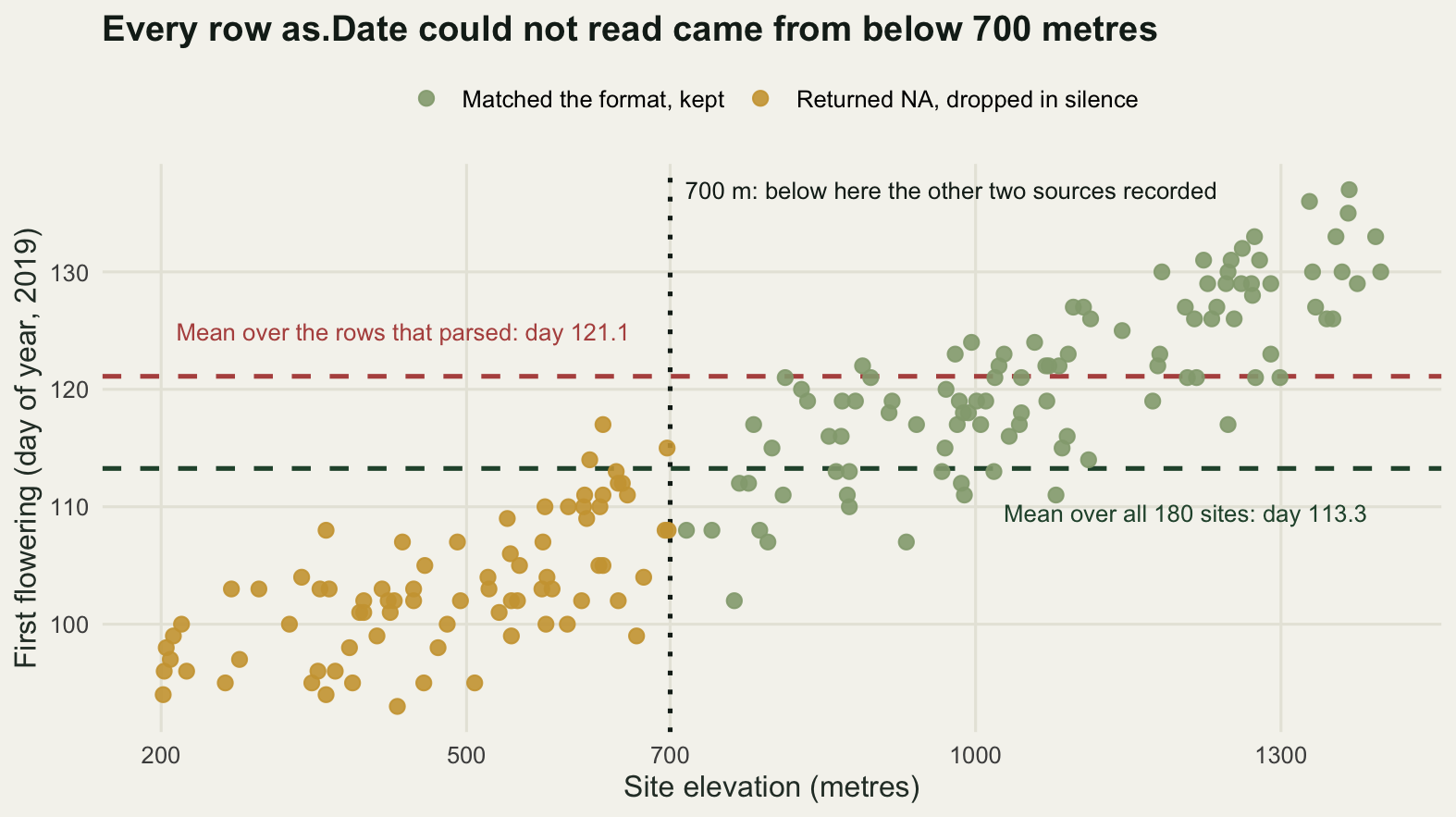
Trying a list of formats, and the trap inside it
The fix is not a longer format string, it is admitting that a merged column has more than one convention in it. A parser that tries several formats in order, records which one worked, and refuses to move on until nothing is left unread takes about a dozen lines.
parse_field_date <- function(x, formats) {
  out <- rep(as.Date(NA), length(x))
  used <- rep(NA_character_, length(x))
  for (f in formats) {
    todo <- which(is.na(out))
    if (!length(todo)) break
    got <- as.Date(x[todo], format = f)
    ok <- !is.na(got)
    out[todo[ok]] <- got[ok]
    used[todo[ok]] <- f
  }
  list(date = out, format = used)
}

careless <- parse_field_date(written_2019, c("%Y-%m-%d", "%d/%m/%Y", "%d.%m.%Y"))
careful  <- parse_field_date(written_2019, c("%Y-%m-%d", "%d/%m/%Y", "%d.%m.%y"))
print(table(as.numeric(format(careless$date, "%Y"))))
  19 2019
34 146 print(table(careful$format))
%d.%m.%y %d/%m/%Y %Y-%m-%d
34 44 102 print(c(as.Date("17.04.19", "%d.%m.%Y"), as.Date("17.04.19", "%d.%m.%y"),
as.Date("17.04.68", "%d.%m.%y"), as.Date("17.04.69", "%d.%m.%y")))[1] "0019-04-17" "2019-04-17" "2068-04-17" "1969-04-17"year_careless <- as.numeric(format(careless$date, "%Y"))
round(c(careless_unparsed = sum(is.na(careless$date)),
careless_rows_in_year_19 = sum(year_careless < 1000),
careless_mean_doy = mean(as.numeric(format(careless$date, "%j"))),
careless_span_days = as.numeric(diff(range(careless$date))),
careful_unparsed = sum(is.na(careful$date)),
careful_rows_matching_truth = sum(careful$date == d_2019),
careful_change_days = mean(as.numeric(format(careful$date, "%j"))) -
mean(doy_2018),
rows_flagged_by_a_year_range_check = sum(year_careless != 2019)), 4) careless_unparsed careless_rows_in_year_19
0.0000 34.0000
careless_mean_doy careless_span_days
113.2611 730529.0000
careful_unparsed careful_rows_matching_truth
0.0000 180.0000
careful_change_days rows_flagged_by_a_year_range_check
-1.5778 34.0000 The careful list gets everything: 0 rows unparsed, all 180 dates identical to the truth, and the year-on-year change back to an advance of 1.5778 days. The table of which format matched which row is worth printing every time, because it is the cheapest possible summary of what your file actually contains: 102 ISO strings, 44 with slashes, 34 with dots.
The careless list is the interesting one. It differs by a single character, %Y where the data have a two-digit year, and it also reports 0 rows unparsed. %Y will happily read 19 as the year 19, so 17.04.19 becomes the seventeenth of April in the year 19, two thousand years before the survey. Nothing about that is flagged. The mean day of year comes out at 113.2611, exactly the same as the correct parse, because the day and the month were read correctly and only the year is absurd. Any analysis that works in day of year sails straight past it. The moment you subtract two dates, the span of the column is 730529 days.
The two-digit year has a second trap sitting behind the first. %y does not mean “the current century”: R applies a window, and 68 reads as 2068 while 69 reads as 1969. For a phenology series that is a difference of ninety-nine years in a single character.
Both are caught by the same thing, and it is not a cleverer format string. It is a range check on the parsed result: every date in a 2019 survey should have the year 2019. That check flags all 34 of the bad rows, costs one line, and would have caught the century window as well.
# not run here, because this post has to render with nothing installed beyond
# ggplot2.  The lubridate package covers most of the above:
library(lubridate)
dmy("17/04/2019")                  # order by name rather than by format string
parse_date_time(written_2019, orders = c("Ymd", "dmy"))   # separators ignored
year(dmy("17.04.19"))              # 2019, but 17.04.68 is 2068 by the same window
The parse that succeeds and is wrong
An NA is a bad outcome with a good property: it is visible if you count it. The failure with no outcome at all is the day and the month arriving in the other order, because for a large part of the calendar both readings are legal dates.
all_2019 <- seq(as.Date("2019-01-01"), as.Date("2019-12-31"), by = "day")
dom <- as.numeric(format(all_2019, "%d"))
mon <- as.numeric(format(all_2019, "%m"))
round(c(days_in_the_year = length(all_2019),
        both_readings_valid = sum(dom <= 12),
        both_readings_valid_percent = 100 * mean(dom <= 12),
        transpose_to_themselves = sum(dom == mon),
        genuinely_damaging = sum(dom <= 12 & dom != mon),
        genuinely_damaging_percent = 100 * mean(dom <= 12 & dom != mon),
        rows_needed_to_expose_the_swap = 1 / (1 - mean(dom <= 12))), 4)
days_in_the_year both_readings_valid
365.0000 144.0000
both_readings_valid_percent transpose_to_themselves
39.4521 12.0000
genuinely_damaging genuinely_damaging_percent
132.0000 36.1644
rows_needed_to_expose_the_swap
1.6516 144 of the 365 days of 2019, 39.4521 per cent, have a day of the month of 12 or less and therefore read as a valid date under either convention. Twelve of those transpose to themselves, the twelfth of December and its eleven siblings, which leaves 132 days, 36.1644 per cent of the year, on which a swap changes the date and produces no complaint.
On data spread through the season this is a mistake that announces itself. Take the 44 slash-format records from the survey above and read them with the month first.
slash <- written_2019[source_2019 == "partner"]
as_written <- as.Date(slash, format = "%d/%m/%Y")
as_swapped <- as.Date(slash, format = "%m/%d/%Y")
round(c(slash_rows = length(slash),
        swapped_to_na = sum(is.na(as_swapped)),
        swapped_to_na_percent = 100 * mean(is.na(as_swapped)),
        swapped_silently = sum(!is.na(as_swapped)),
        swapped_silently_percent = 100 * mean(!is.na(as_swapped)),
        mean_doy_as_written = mean(as.numeric(format(as_written, "%j"))),
        mean_doy_of_the_survivors =
          mean(as.numeric(format(as_swapped, "%j")), na.rm = TRUE)), 4)
slash_rows swapped_to_na swapped_to_na_percent
44.0000 30.0000 68.1818
swapped_silently swapped_silently_percent mean_doy_as_written
14.0000 31.8182 105.6364
mean_doy_of_the_survivors
270.5000 30 of the 44 rows, 68.1818 per cent, come back as NA because there is no month 13 or 27. That is a signature you cannot miss if you count your NA values, and it is why a swapped day and month is usually a five-minute problem on a full season of field dates. If your dates are scattered across the calendar, the calendar itself is the check. Under random sampling you expect to hit an unambiguous date after 1.6516 rows.
The mistake becomes expensive when the survey design removes that protection. A butterfly transect walked once in the first days of the month and once around the tenth has, by construction, no day of the month above 12.
set.seed(20260818)
visit_month <- rep(3:10, each = 2)
visit_day <- as.integer(rep(c(3, 10), 8) + sample(-2:2, 16, replace = TRUE))
visit_day <- pmin(pmax(visit_day, 1), 12)
visit <- as.Date(sprintf("2019-%02d-%02d", visit_month, visit_day))
flight_peak <- as.Date("2019-07-14")
count <- round(190 * exp(-0.5 * (as.numeric(visit - flight_peak) / 19)^2)) + 1
recorded <- format(visit, "%d/%m/%Y")

walked <- as.Date(recorded, format = "%d/%m/%Y")
guessed <- as.Date(recorded, format = "%m/%d/%Y")
print(data.frame(recorded, count, read_as = as.character(guessed)))
recorded count read_as
1 03/03/2019 1 2019-03-03
2 10/03/2019 1 2019-10-03
3 01/04/2019 1 2019-01-04
4 08/04/2019 1 2019-08-04
5 03/05/2019 1 2019-03-05
6 10/05/2019 2 2019-10-05
7 02/06/2019 18 2019-02-06
8 08/06/2019 33 2019-08-06
9 04/07/2019 166 2019-04-07
10 10/07/2019 187 2019-10-07
11 01/08/2019 122 2019-01-08
12 08/08/2019 81 2019-08-08
13 04/09/2019 5 2019-04-09
14 09/09/2019 3 2019-09-09
15 02/10/2019 1 2019-02-10
16 11/10/2019 1 2019-11-10wmean_date <- function(d, w) sum(as.numeric(d) * w) / sum(w)
as_day <- function(v) as.Date(round(v), origin = "1970-01-01")
wm_walked <- wmean_date(walked, count)
wm_guessed <- wmean_date(guessed, count)
pair_flip <- function(a, b) {
ij <- upper.tri(diag(length(a)))
100 * mean(outer(a, a, "-")[ij] * outer(b, b, "-")[ij] < 0)
}
print(c(as.character(as_day(wm_walked)), as.character(as_day(wm_guessed))))[1] "2019-07-14" "2019-06-06"round(c(visits = length(visit),
rows_returning_na = sum(is.na(guessed)),
dates_changed = sum(walked != guessed),
dates_unchanged = sum(walked == guessed),
peak_count = max(count),
weighted_mean_doy_walked = as.numeric(format(as_day(wm_walked), "%j")),
weighted_mean_doy_guessed = as.numeric(format(as_day(wm_guessed), "%j")),
weighted_mean_shift_days = wm_guessed - wm_walked,
busiest_visit_doy_walked =
as.numeric(format(walked[which.max(count)], "%j")),
busiest_visit_doy_guessed =
as.numeric(format(guessed[which.max(count)], "%j")),
largest_single_move_days = max(abs(as.numeric(guessed - walked))),
season_span_walked = as.numeric(diff(range(walked))),
season_span_guessed = as.numeric(diff(range(guessed))),
visit_pairs_out_of_order_percent =
pair_flip(as.numeric(walked), as.numeric(guessed)),
spearman = cor(as.numeric(walked), as.numeric(guessed),
method = "spearman")), 4) visits rows_returning_na
16.0000 0.0000
dates_changed dates_unchanged
13.0000 3.0000
peak_count weighted_mean_doy_walked
187.0000 195.0000
weighted_mean_doy_guessed weighted_mean_shift_days
157.0000 -37.7965
busiest_visit_doy_walked busiest_visit_doy_guessed
191.0000 280.0000
largest_single_move_days season_span_walked
234.0000 222.0000
season_span_guessed visit_pairs_out_of_order_percent
310.0000 40.0000
spearman
0.2471 Sixteen visits, 0 rows returning NA, no warning of any kind, and 13 of the 16 dates are now a different day. The 3 that survive are the ones where the day and the month happen to be equal.
The abundance-weighted mean flight date, which is the quantity a transect scheme reports, moves from 14 July to 6 June: day 195 becomes day 157, a shift of 37.7965 days. That is more than an order of magnitude larger than any published decadal trend in butterfly flight periods, and it is produced by a data-reading step nobody wrote down. The busiest visit of the year, the one with 187 individuals, moves from day 191 to day 280, so the flight curve now peaks in October. The largest single date moves 234 days. The visits are no longer in the order they were walked: 40 per cent of visit pairs come out the wrong way round and the rank correlation between the walked dates and the read dates is 0.2471.
lev <- c("As read, month first", "As written, day first")
swap_df <- data.frame(
  date = c(walked, guessed), count = rep(count, 2),
  row = factor(rep(c("As written, day first", "As read, month first"), each = 16),
               levels = lev))
seg_df <- data.frame(x = walked, xend = guessed,
                     y = factor("As written, day first", levels = lev),
                     yend = factor("As read, month first", levels = lev))
peak <- which.max(count)
peak_df <- seg_df[peak, ]

ggplot(swap_df, aes(date, row)) +
  geom_segment(data = seg_df, aes(x = x, xend = xend, y = y, yend = yend),
               inherit.aes = FALSE, colour = te_pal$line, linewidth = 0.8) +
  geom_segment(data = peak_df, aes(x = x, xend = xend, y = y, yend = yend),
               inherit.aes = FALSE, colour = te_pal$ink, linewidth = 0.9) +
  geom_vline(xintercept = as_day(wm_walked), linetype = 2, colour = te_pal$forest,
             linewidth = 0.9) +
  geom_vline(xintercept = as_day(wm_guessed), linetype = 2, colour = te_pal$clay,
             linewidth = 0.9) +
  geom_point(aes(size = count, colour = row), alpha = 0.9) +
  annotate("text", x = guessed[peak] - 4, y = 2.46, hjust = 1, size = 3.3,
           colour = te_pal$ink,
           label = "the busiest visit, 187 butterflies, reads as 7 Oct") +
  annotate("text", x = walked[peak], y = 0.76, hjust = 0.5, size = 3.3,
           colour = te_pal$ink, label = "the same visit as written: 10 Jul") +
  annotate("text", x = as_day(wm_guessed) - 4, y = 0.36, hjust = 1, size = 3.3,
           colour = te_pal$clay, label = "weighted mean as read: 6 Jun") +
  annotate("text", x = as_day(wm_walked) + 4, y = 0.36, hjust = 0, size = 3.3,
           colour = te_pal$forest, label = "weighted mean as written: 14 Jul") +
  scale_colour_manual(values = c(te_pal$clay, te_pal$forest), guide = "none") +
  scale_size_area(max_size = 8, name = "Butterflies counted",
                  breaks = c(1, 50, 100, 187)) +
  scale_y_discrete(expand = expansion(add = c(1.15, 1.05))) +
  scale_x_date(date_labels = "%b", date_breaks = "2 months") +
  labs(x = "Date in 2019", y = NULL,
       title = "Sixteen visits, no warnings, and the flight peak lands in October") +
  theme_te() +
  theme(legend.position = "top",
        axis.text.y = element_text(colour = te_pal$ink, size = 10))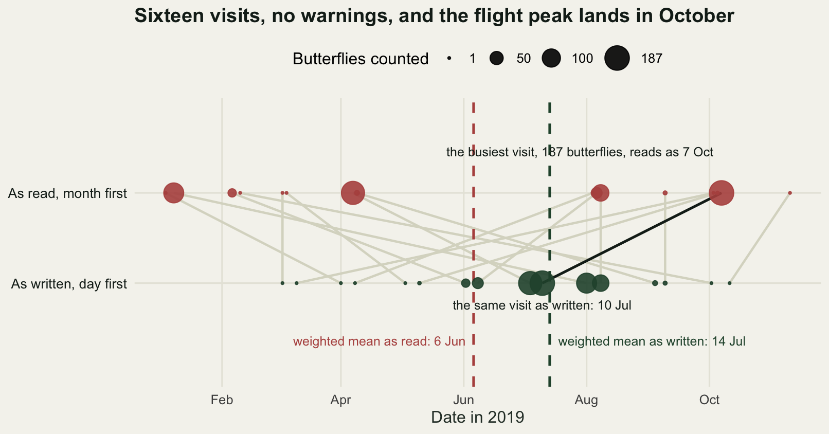
There is a check for this, and it is short enough to run on every date column you ever open. Read the column under both conventions and count what each row allows: a row that parses one way and not the other decides the convention for the whole column, a row that parses both ways decides nothing, and a row that parses neither way is a different problem.
date_convention <- function(x) {
  day_first <- as.Date(x, format = "%d/%m/%Y")
  month_first <- as.Date(x, format = "%m/%d/%Y")
  c(rows = length(x),
    decides_day_first = sum(!is.na(day_first) & is.na(month_first)),
    decides_month_first = sum(is.na(day_first) & !is.na(month_first)),
    allows_either = sum(!is.na(day_first) & !is.na(month_first)),
    allows_neither = sum(is.na(day_first) & is.na(month_first)))
}
print(rbind(survey_column = date_convention(slash),
            transect_column = date_convention(recorded)))
rows decides_day_first decides_month_first allows_either
survey_column 44 30 0 14
transect_column 16 0 0 16
allows_neither
survey_column 0
transect_column 0The two columns give opposite answers. The survey column has 30 rows that can only be read with the day first and 14 that go either way, so the convention is settled by the file itself and the remaining 14 rows come along for the ride. The transect column has 0 rows that decide anything and all 16 that go either way. That is not a warning and not an error, it is a fact about the data: the information required to read the column is not in the column. Somebody has to supply it, and if nobody does, the analysis proceeds on a guess.
Running that four-number summary is the difference between a five-minute problem and a retracted flight period. It costs nine lines and it is the only check in this post that can tell you, before you have any results to compare against, that you are about to guess.
The general lesson is not “always use the day first”. It is that a date column has a convention, the convention is not written in the file, and the only way to establish it is to look for a row that can only be read one way. When the design guarantees there is no such row, the column has to carry its convention some other way: a written note, a separate column, or a rewrite into ISO order at the point of entry, which is why every guide to spreadsheet hygiene asks for 2019-07-04 and means it.
A clock reading is not an instant
Dates are the easy half. A timestamp adds a time zone, and a time zone that observes summer time is not a constant offset. Two consequences follow, and both are silent.
tz_site <- "Europe/Budapest"
minute_of_march <- seq(as.POSIXct("2019-03-30 23:00:00", tz = "UTC"),
                       as.POSIXct("2019-03-31 22:59:00", tz = "UTC"), by = "min")
minute_of_october <- seq(as.POSIXct("2019-10-26 22:00:00", tz = "UTC"),
                         as.POSIXct("2019-10-27 22:59:00", tz = "UTC"), by = "min")
local_march <- format(minute_of_march, "%Y-%m-%d %H:%M", tz = tz_site)
local_october <- format(minute_of_october, "%Y-%m-%d %H:%M", tz = tz_site)
march_day <- local_march[substr(local_march, 1, 10) == "2019-03-31"]
october_day <- local_october[substr(local_october, 1, 10) == "2019-10-27"]

t1 <- as.POSIXct("2019-03-31 01:40:00", tz = tz_site)
t2 <- as.POSIXct("2019-03-31 03:20:00", tz = tz_site)
clock_gap <- (3 + 20 / 60) - (1 + 40 / 60)
round(c(minutes_in_31_march = length(march_day),
        distinct_clock_readings_31_march = length(unique(march_day)),
        clock_readings_naming_no_instant = 1440 - length(unique(march_day)),
        minutes_in_27_october = length(october_day),
        distinct_clock_readings_27_october = length(unique(october_day)),
        clock_readings_naming_two_instants = sum(table(october_day) > 1),
        clock_difference_hours = clock_gap,
        elapsed_hours = as.numeric(difftime(t2, t1, units = "hours")),
        overstated_by_minutes =
          60 * (clock_gap - as.numeric(difftime(t2, t1, units = "hours")))), 4)
minutes_in_31_march distinct_clock_readings_31_march
1380.0000 1380.0000
clock_readings_naming_no_instant minutes_in_27_october
60.0000 1500.0000
distinct_clock_readings_27_october clock_readings_naming_two_instants
1440.0000 60.0000
clock_difference_hours elapsed_hours
1.6667 0.6667
overstated_by_minutes
60.0000 The map from wall clock readings to instants is not one to one, twice a year. On 31 March 2019 the local day in this zone is 1380 minutes long, and 60 clock readings, the ones from 02:00 to 02:59, name no instant at all. On 27 October the day is 1500 minutes long and there are only 1440 distinct readings, so 60 of them each name two different instants an hour apart. A timestamp written as 2019-10-27 02:30:00 with no zone is not an ambiguous label for one moment: it is a label for two.
The arithmetic follows from that. A camera fires at 01:40 and again at 03:20 on 31 March. Subtract the clock readings and you get 1.6667 hours. The instants are 0.6667 hours apart. The clock overstates the interval by exactly 60 minutes, and difftime on properly constructed POSIXct values gets it right without being asked, because it works on instants rather than on the digits.
The autumn half is worse, because there is nothing to detect. Two instants a full hour apart are written down as the same string.
pair <- as.POSIXct(c("2019-10-27 00:30:00", "2019-10-27 01:30:00"), tz = "UTC")
print(format(pair, "%Y-%m-%d %H:%M:%S", tz = tz_site))
[1] "2019-10-27 02:30:00" "2019-10-27 02:30:00"round(c(distinct_utc_instants = length(unique(pair)),
distinct_local_strings =
length(unique(format(pair, "%Y-%m-%d %H:%M:%S", tz = tz_site))),
hours_between_the_instants =
as.numeric(difftime(pair[2], pair[1], units = "hours"))), 4) distinct_utc_instants distinct_local_strings
2 1
hours_between_the_instants
1 2 instants, 1 local string, 1 hour apart. Whichever way a parser resolves 2019-10-27 02:30:00, one of those two detections is being placed an hour from where it happened, and no rule recovers which one, because the file no longer contains the difference. This is the argument for storing instants in UTC and keeping the local zone in its own column: UTC has no repeated readings and no missing ones, so the mapping stays one to one and the local clock can always be reconstructed from it. The reverse is not true.
There is a third silent behaviour in the same family, and it has nothing to do with summer time. difftime chooses its units from the size of the gap unless you name them.
short <- as.POSIXct("2019-05-04 06:30:00", tz = "UTC")
gaps <- c(45, 90, 5400, 200000)
print(data.frame(seconds = gaps,
                 auto_units = sapply(gaps, function(g)
                   attr(difftime(short + g, short), "units")),
                 auto_value = sapply(gaps, function(g)
                   as.numeric(difftime(short + g, short))),
                 forced_hours = round(sapply(gaps, function(g)
                   as.numeric(difftime(short + g, short), units = "hours")), 4)))
seconds auto_units auto_value forced_hours
1 45 secs 45.000000 0.0125
2 90 mins 1.500000 0.0250
3 5400 hours 1.500000 1.5000
4 200000 days 2.314815 55.5556A gap of 90 seconds and a gap of 5400 seconds both come back from as.numeric as 1.5. One is a minute and a half, the other is an hour and a half, and the two differ by a factor of 60. Nothing in the number says which. The habit that removes the problem is to write the units into every difftime call, units = "hours" or units = "days", and never to call as.numeric on a difference whose units were chosen for you.
It matters most on a series of gaps rather than on one gap. A single call picks one unit for the whole vector, but gaps computed one call at a time, the way the chunk above does, or split by group, cross the threshold partway through, so some entries end up in minutes and some in hours with no marker between them.
Every failure so far in this section is one interval, or one pair of instants. The version that damages a published result is a series.
set.seed(20260818)
n_night <- 62
per_night <- 9
night_one <- as.Date("2019-03-01")
inst <- unlist(lapply(seq_len(n_night), function(k) {
  midnight <- as.numeric(as.POSIXct(paste0(night_one + k - 1, " 00:00:00"),
                                    tz = "UTC"))
  midnight + 3600 * rnorm(per_night, 19.5 + (1 / 60) * (k - 1), 0.35)
}))
inst <- as.POSIXct(inst, origin = "1970-01-01", tz = "UTC")
logged <- format(inst, "%Y-%m-%d %H:%M:%S", tz = tz_site)
print(head(logged, 4))
[1] "2019-03-01 19:41:16" "2019-03-01 20:11:12" "2019-03-01 20:13:26"
[4] "2019-03-01 20:52:43"That is 62 nights of a nocturnal mammal at a camera trap, from 1 March to 1 May 2019. The animal emerges at a fixed point in solar time, here 19:30 UTC on the first night, and that point drifts one minute later per night through the spring, which is roughly how a species tracking sunset behaves at this latitude. Over the 62 nights of the study that is a real drift of about an hour. The camera writes local wall clock text, because that is what cameras do.
The naive analysis reads the hour and minute straight out of the string. The careful one hands the string back to R with the zone it was written in, and asks for the instant.
hour_of <- function(s) as.numeric(substr(s, 12, 13)) +
  as.numeric(substr(s, 15, 16)) / 60 + as.numeric(substr(s, 18, 19)) / 3600
clock_hour <- hour_of(logged)
recovered <- as.POSIXct(logged, tz = tz_site)
recovered_hour <- hour_of(format(recovered, "%Y-%m-%d %H:%M:%S", tz = "UTC"))
true_hour <- hour_of(format(inst, "%Y-%m-%d %H:%M:%S", tz = "UTC"))
night_index <- rep(seq_len(n_night), each = per_night)
after <- inst >= as.POSIXct("2019-03-31 01:00:00", tz = "UTC")

b_clock <- coef(lm(clock_hour ~ night_index))[2]
b_true <- coef(lm(true_hour ~ night_index))[2]
b_recovered <- coef(lm(recovered_hour ~ night_index))[2]
round(c(detections = length(inst), nights = n_night,
        before_the_change = sum(!after), after_the_change = sum(after),
        clock_sd_hours = sd(clock_hour), true_sd_hours = sd(true_hour),
        sd_inflation = sd(clock_hour) / sd(true_hour),
        mean_clock_hour_before = mean(clock_hour[!after]),
        mean_clock_hour_after = mean(clock_hour[after]),
        clock_step_minutes = 60 * (mean(clock_hour[after]) -
                                     mean(clock_hour[!after])),
        true_step_minutes = 60 * (mean(true_hour[after]) -
                                    mean(true_hour[!after])),
        reported_drift_minutes = 60 * b_clock * (n_night - 1),
        true_drift_minutes = 60 * b_true * (n_night - 1),
        recovered_drift_minutes = 60 * b_recovered * (n_night - 1),
        overstatement_factor = b_clock / b_true,
        overstated_by_minutes = 60 * (b_clock - b_true) * (n_night - 1),
        busiest_true_hour_percent =
          100 * max(table(floor(true_hour))) / length(true_hour),
        busiest_clock_hour_percent =
          100 * max(table(floor(clock_hour))) / length(clock_hour),
        detections_recovered_exactly =
          sum(abs(recovered_hour - true_hour) < 1e-6)), 4)
detections nights
558.0000 62.0000
before_the_change after_the_change
270.0000 288.0000
clock_sd_hours true_sd_hours
0.8540 0.4715
sd_inflation mean_clock_hour_before
1.8112 20.7472
mean_clock_hour_after clock_step_minutes
22.2604 90.7920
true_step_minutes reported_drift_minutes.night_index
30.7920 150.6469
true_drift_minutes.night_index recovered_drift_minutes.night_index
62.1676 62.1676
overstatement_factor.night_index overstated_by_minutes.night_index
2.4232 88.4793
busiest_true_hour_percent busiest_clock_hour_percent
49.4624 36.7384
detections_recovered_exactly
558.0000 print(table(floor(clock_hour)))
 19  20  21  22  23
5 194 150 205 4 print(table(floor(true_hour)))
 18  19  20  21
  5 273 276   4
558 detections over 62 nights, 270 of them before the clocks went forward and 288 after. The finding is the seasonal drift, because that is what the study is for. In real time the animal moved 62.1676 minutes later across the study. Read off the clock digits, it moved 150.6469 minutes later: an overstatement of 88.4793 minutes, a factor of 2.4232. Roughly an hour of the reported effect is a legislative artefact rather than a behavioural one, and it arrives on one night in the middle of the series.
Read off the wall clock the mean emergence time is 20.7472 before the change and 22.2604 after, a jump of 90.7920 minutes where the instants moved only 30.7920. The spread inflates with it: the standard deviation of emergence time is 0.4715 hours on the real instants and 0.8540 on the clock readings, an inflation of 1.8112, and the busiest whole hour holds 49.4624 per cent of detections in real time against 36.7384 per cent on the clock. A species with one sharp emergence peak is reported as a species with a broad one.
The repair is one function call. Parsing the same strings with tz = "Europe/Budapest" and reading them back in UTC recovers all 558 instants exactly, and the estimated drift returns to 62.1676 minutes. R already holds the rules; it simply will not guess which zone the text came from.
clock_df <- data.frame(
  night = rep(night_index, 2), hour = c(clock_hour, true_hour),
  series = factor(rep(c("Wall clock text in the file",
                        "The same instants in UTC"), each = length(clock_hour)),
                  levels = c("Wall clock text in the file",
                             "The same instants in UTC")))
fit_df <- data.frame(
  intercept = c(coef(lm(clock_hour ~ night_index))[1],
                coef(lm(true_hour ~ night_index))[1]),
  slope = c(b_clock, b_true),
  series = factor(levels(clock_df$series), levels = levels(clock_df$series)))

ggplot(clock_df, aes(night, hour, colour = series)) +
  geom_vline(xintercept = 31, linetype = 2, colour = te_pal$sage,
             linewidth = 0.9) +
  geom_point(size = 1.5, alpha = 0.45) +
  geom_abline(data = fit_df, aes(intercept = intercept, slope = slope,
                                 colour = series),
              linewidth = 1.1, show.legend = FALSE) +
  annotate("text", x = 32.4, y = 18.35, hjust = 0, size = 3.3,
           colour = te_pal$ink, label = "clocks go forward, 31 March") +
  scale_colour_manual(values = c(te_pal$clay, te_pal$forest), name = NULL) +
  scale_y_continuous(breaks = seq(18, 24, 1)) +
  labs(x = "Night of the study (1 March to 1 May 2019)",
       y = "Time of emergence (hours)",
       title = "A 62 minute seasonal drift is reported as 151 minutes") +
  theme_te() +
  theme(legend.position = "top")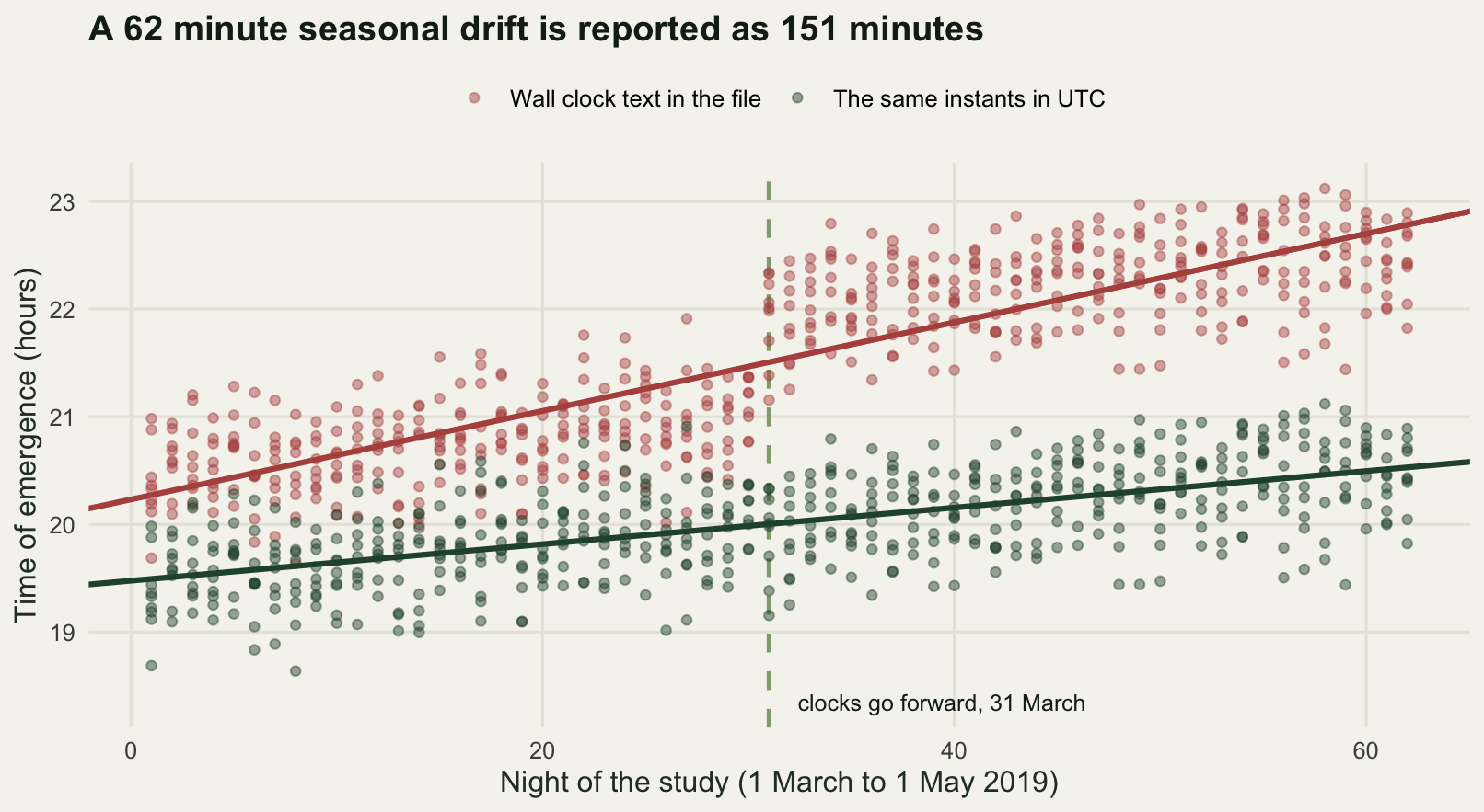
A year is not 365 days
The last failure needs no bad data at all. It is arithmetic, and it comes from the most reasonable line in the script.
spans <- c(1, 2, 4, 5, 10, 20, 50)
print(round(t(sapply(spans, function(s) {
  a <- as.Date("2001-04-18")
  b <- as.Date(paste0(2001 + s, "-04-18"))
  c(years = s, real_days = as.numeric(b - a), times_365 = 365 * s,
    out_by = as.numeric(b - a) - 365 * s,
    out_by_using_365.25 = as.numeric(b - a) - 365.25 * s)
})), 4))
years real_days times_365 out_by out_by_using_365.25
[1,] 1 365 365 0 -0.25
[2,] 2 730 730 0 -0.50
[3,] 4 1461 1460 1 0.00
[4,] 5 1826 1825 1 -0.25
[5,] 10 3652 3650 2 -0.50
[6,] 20 7305 7300 5 0.00
[7,] 50 18262 18250 12 -0.50cycle_days <- as.numeric(as.Date("2401-01-01") - as.Date("2001-01-01"))
is_leap <- function(y) (y %% 4 == 0 & y %% 100 != 0) | y %% 400 == 0
print(round(c(days_in_one_400_year_cycle = cycle_days,
leap_years_in_the_cycle = sum(is_leap(2001:2400)),
mean_year_days = cycle_days / 400), 4))days_in_one_400_year_cycle leap_years_in_the_cycle
146097.0000 97.0000
mean_year_days
365.2425 print(seq(as.Date("2020-01-31"), by = "month", length.out = 5))[1] "2020-01-31" "2020-03-02" "2020-03-31" "2020-05-01" "2020-05-31"print(as.Date(c("2019-02-29", "2019-04-31"), format = "%Y-%m-%d"))[1] NA NAThe same calendar date twenty years apart is 7305 days away, not 7300. Over fifty years the gap is 12 days. The reason is in the second block: one full Gregorian cycle of 400 years runs to 146097 days and contains 97 leap years, so the mean length of a year in this calendar is 365.2425 days. Multiplying by 365 loses a quarter of a day every year and pays it back in whole days at unpredictable moments. Using 365.25 instead stays under a day out for any span shorter than a century, which is close enough for most purposes and wrong in a different way at the century boundaries, where the Gregorian rule drops a leap year that 365.25 keeps.
Two other pieces of calendar arithmetic in the same block are worth seeing. Adding a month to 31 January 2020 by seq gives 2 March, because there is no 31 February and the sequence is generated by adding month numbers and letting the result normalise. And as.Date returns NA for both 2019-02-29 and 2019-04-31, silently, which is one more argument for the range check: a non-existent date is indistinguishable from an unreadable one once it is NA.
Now what that does to a phenological trend. Twenty seasons of a first-flowering date, 2001 to 2020. The interesting question is whether flowering is getting earlier, in days per decade. The simulated series is built so that the answer is known: the year-to-year wobble is drawn and then residualised against year, so the first series has exactly no trend before rounding, and the second has a real advance of 2.8 days per decade added to the same wobble.
set.seed(20260818)
season <- 2001:2020
k <- season - 2001
anniversary <- as.Date(paste0(season, "-04-18"))
wobble <- round(residuals(lm(rnorm(length(season), 0, 3.0) ~ k)))
flat_dates <- anniversary + wobble
advance_per_year <- 0.28
advancing_dates <- anniversary + round(wobble - advance_per_year * k)

trend_pair <- function(d) {
  correct <- as.numeric(d - anniversary)
  naive <- as.numeric(d - d[1]) - 365 * k
  a <- summary(lm(correct ~ k))$coefficients[2, ]
  b <- summary(lm(naive ~ k))$coefficients[2, ]
  c(calendar_trend = 10 * a[1], calendar_p = a[4],
    naive_trend = 10 * b[1], naive_p = b[4])
}
leap_days <- as.numeric(anniversary - anniversary[1]) - 365 * k
print(round(rbind(no_real_trend = trend_pair(flat_dates),
                  real_advance = trend_pair(advancing_dates)), 4))
calendar_trend.Estimate calendar_p.Pr(>|t|) naive_trend.Estimate
no_real_trend 0.0602 0.9569 2.5789
real_advance -2.6541 0.0253 -0.1353
naive_p.Pr(>|t|)
no_real_trend 0.0291
real_advance 0.9020round(c(seasons = length(season),
built_in_advance_days_per_decade = 10 * advance_per_year,
leap_days_over_the_series = leap_days[20],
leap_drift_days_per_decade = 10 * coef(lm(leap_days ~ k))[2],
real_elapsed_days = as.numeric(anniversary[20] - anniversary[1]),
naive_elapsed_days = 365 * 19), 4) seasons built_in_advance_days_per_decade
20.0000 2.8000
leap_days_over_the_series leap_drift_days_per_decade.k
5.0000 2.5188
real_elapsed_days naive_elapsed_days
6940.0000 6935.0000 The two ways of expressing “how much later than the first season did it flower” look equally sensible. The calendar version subtracts the same date in each year, as.Date(paste0(season, "-04-18")), which is exact by construction. The naive version subtracts the first record’s date and then removes 365 days per elapsed year, which is the line you write when you want to strip out the whole years and keep the remainder.
Over 2001 to 2020 the anniversary is 6940 days away and 365 times 19 is 6935, so the naive subtraction leaves 5 extra days lying in the response. They do not arrive smoothly: they arrive in 2004, 2008, 2012, 2016 and 2020, which as a function of year is a staircase with an average slope of 2.5188 days per decade. That slope goes straight into the regression.
In the series built to have no trend, the calendar version reports 0.0602 days per decade with a p value of 0.9569, which is the right answer. The naive version reports a delay of 2.5789 days per decade with a p value of 0.0291. A phenological signal that clears the conventional cutoff on this run, in a series that by construction contains none, from a data set with no missing values, no bad dates and no outliers.
In the series with a real advance of 2.8 days per decade, the calendar version recovers it at -2.6541 days per decade, p equals 0.0253. The naive version reports -0.1353 days per decade with a p value of 0.9020: no trend, nothing to report, the study writes itself up as a null result. One constant, two opposite errors, and in neither case does anything in the output look wrong.
panel_df <- function(d, lab) {
  correct <- as.numeric(d - anniversary)
  naive <- as.numeric(d - d[1]) - 365 * k
  data.frame(season = rep(season, 2),
             value = c(correct - correct[1], naive - naive[1]),
             method = rep(c("Exact calendar difference",
                            "365 days per elapsed year"), each = length(season)),
             panel = lab)
}
lab_a <- "A series with no real trend"
lab_b <- sprintf("A series advancing %.1f days per decade", 10 * advance_per_year)
leap_df <- rbind(panel_df(flat_dates, lab_a), panel_df(advancing_dates, lab_b))
leap_df$panel <- factor(leap_df$panel, levels = c(lab_a, lab_b))
leap_df$method <- factor(leap_df$method,
                         levels = c("Exact calendar difference",
                                    "365 days per elapsed year"))

ggplot(leap_df, aes(season, value, colour = method)) +
  geom_hline(yintercept = 0, colour = te_pal$line, linewidth = 0.8) +
  geom_point(size = 2.3, alpha = 0.9) +
  stat_smooth(method = "lm", formula = y ~ x, se = FALSE, linewidth = 1.1) +
  facet_wrap(~panel) +
  scale_colour_manual(values = c(te_pal$forest, te_pal$clay), name = NULL) +
  labs(x = "Season", y = "Days later than the first season",
       title = "One wrong constant invents a trend, then hides a real one") +
  theme_te() +
  theme(legend.position = "top",
        strip.text = element_text(colour = te_pal$ink, face = "bold", size = 9))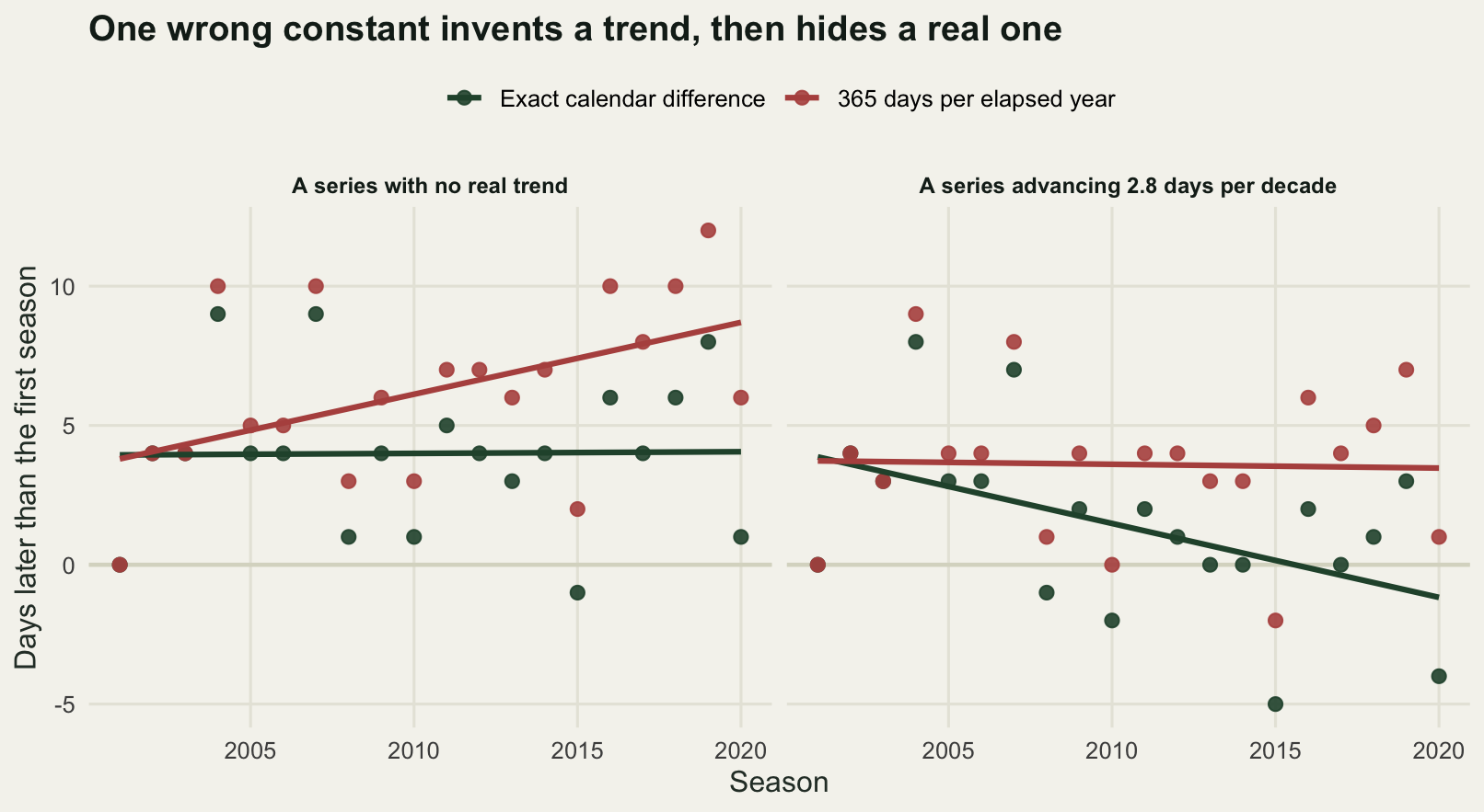
# not run here.  lubridate's month arithmetic keeps the day of the month where
# base R lets it overflow:
library(lubridate)
ymd("2020-01-31") %m+% months(1)        # 2020-02-29, not 2020-03-02
ymd("2020-03-31") %m-% months(1)        # 2020-02-29, rolled back the same way
The honest limit
Everything above assumes each source is internally consistent: the partner network always writes the day first, the volunteers always use dots. That assumption is doing a great deal of work, and where it fails there is no measurement in this post that helps.
set.seed(20260818)
retyped <- sample(seq_along(slash), 11)
mixed <- slash
mixed[retyped] <- format(as_written[retyped], "%m/%d/%Y")
one_format <- as.Date(mixed, format = "%d/%m/%Y")
round(c(column_rows = length(mixed),
        rows_retyped = length(retyped),
        retyped_rows_flagged_as_na = sum(is.na(one_format[retyped])),
        retyped_rows_read_silently = sum(!is.na(one_format[retyped])),
        mean_error_on_the_silent_rows_days =
          mean(abs(as.numeric(one_format[retyped] - as_written[retyped])),
               na.rm = TRUE),
        untouched_rows_still_correct =
          sum(one_format[-retyped] == as_written[-retyped])), 4)
column_rows rows_retyped
44 11
retyped_rows_flagged_as_na retyped_rows_read_silently
9 2
mean_error_on_the_silent_rows_days untouched_rows_still_correct
103 33 Eleven of the 44 slash rows are re-typed in the other order, the way a column looks after two people have edited it. Reading the column with one format gets 33 untouched rows right and flags 9 of the 11 as NA, which is the good case. The remaining 2 are read without complaint and land an average of 103 days from where they belong. A format list cannot fix this, because the file no longer contains the information needed to fix it: the convention is a property of the row, and the row does not say which one it is. The only repair is upstream, in how the data were entered.
Four further limits are worth stating plainly.
The time zone measurement assumes the camera’s clock was set correctly and to the zone the file implies. If the clock was an hour out, or was set to a neighbouring zone, or drifted over the deployment, the file looks exactly the same and nothing here detects it. The transition artefact is findable because it happens on a known date; a mis-set clock is only findable against an external reference, such as a known sunset time or a second logger.
The seasonal drift in the camera trap simulation is a single straight line by construction. Real emergence tracks sunset, which is not linear in date, and the summer time step and the real seasonal change are confounded in a way this simulation does not reproduce. What the measurement shows is the size of the artefact, not that a curve would separate the two.
The zone rules themselves are data. Europe/Budapest has followed the same summer time rule since 1996 and so the numbers here are stable, but many zones have changed their rules within the span of a long ecological series, and the database that R consults is updated. A timestamp stored without a zone can therefore be parsed to one instant this year and a different one next year. Storing the instant in UTC, and the zone as a separate field, is the only version of the data that does not have this problem.
And the leap year arithmetic fixes the elapsed days between two dates. It does not fix the harder question of what the anniversary of an ecological event even is, given that the biological year is not the calendar year. That belongs to phenology in R: day of year and event timing, not here.
Where to go next
The cheapest thing you can do after reading this is to print a table of which format matched which row, every time you read a date column, and a range check on the parsed years. Both are one line. Reading field data into R makes the same argument for the rest of the columns, and shows why an empty cell, a recorded zero and an unvisited plot need to stay distinct all the way through. Once the dates are trustworthy, phenology in R: day of year and event timing is where they turn into event timing.
If your dates arrive inside free text, in a comments column or a filename, the extraction is a pattern-matching job before it is a parsing job, and text and regular expressions in R covers how to measure whether a pattern is pulling out what you think. When the parsing is spread over a long script rather than one line, checking an analysis script and debugging and defensive R code are about finding the point at which a value stopped being what you expected.
References
Grolemund G, Wickham H 2011 Journal of Statistical Software 40(3):1-25 (10.18637/jss.v040.i03)
Broman KW, Woo KH 2018 The American Statistician 72(1):2-10 (10.1080/00031305.2017.1375989)
Ziemann M, Eren Y, El-Osta A 2016 Genome Biology 17:177 (10.1186/s13059-016-1044-7)
Zeileis A, Grothendieck G 2005 Journal of Statistical Software 14(6):1-27 (10.18637/jss.v014.i06)
Fitter AH, Fitter RSR 2002 Science 296(5573):1689-1691 (10.1126/science.1071617)
Michener WK 2015 PLoS Computational Biology 11(10):e1004525 (10.1371/journal.pcbi.1004525)