library(ggplot2)

te_pal <- list(forest = "#275139", green = "#2f8f63", sage = "#93a87f",
               clay = "#b5534e", gold = "#cda23f", line = "#dad9ca",
               ink = "#16241d", paper = "#f5f4ee")

theme_te <- function() {
  theme_minimal(base_size = 12) +
    theme(panel.grid.minor = element_blank(),
          panel.grid.major = element_line(colour = "#e7e6dc"),
          plot.background = element_rect(fill = "#f5f4ee", colour = NA),
          panel.background = element_rect(fill = "#f5f4ee", colour = NA),
          plot.title = element_text(face = "bold", colour = te_pal$ink),
          axis.title = element_text(colour = "#2c3a31"))
}Testing your analysis code
R
reproducibility
ecology tutorial
ggplot2
Write a test runner in base R, then measure it: which kinds of test catch the small coding errors that quietly change an ecological result, and which miss them.
Step 41 of the Tidy Ecology course, Part eight: make the result hold up.
A student hands you a script. It reads a season of quadrat counts, computes richness and diversity for each site, ranks the sites, and draws a figure. It runs without complaint. It has run without complaint every Monday since March, the figure has been in two talks, and at no point has anyone asked the script a question it could fail. That is the situation this post is about: not code that crashes, which announces itself, but code that returns a number of the right shape and the right order of magnitude and the wrong value.
The remedy is a test: a statement about what the code should do, written down in a form that can be run. This post writes the machinery by hand in base R, twenty-odd lines, and then measures it. Two real errors go in first, both taken from field data work: a function that drops missing counts as though they were zeros, and a function that returns per cent where the caller expects a fraction. The main measurement comes after that. Thirty-odd small edits are made to a working diversity function, one at a time, and three kinds of test are scored on two things: how many of the edits they catch, and how many lines of test code that costs.
The missing value example leans on reading field data into R, which argues that an empty cell, a recorded zero and a plot nobody visited are three different things. Here that argument turns into something sharper: a check that either passes or fails.
A test runner in twenty lines of base R
A test framework has to do four things: state an expectation, decide whether it held, keep a record, and report at the end. All four fit in a handful of base R functions. The comparison helper is the fiddly part, because floating point equality is not equality, and because a check that throws an error should be recorded as a failure rather than stopping the run.
run_new <- function() data.frame(check = character(0), passed = logical(0),
                                 stringsAsFactors = FALSE)

expect <- function(run, check, condition) {
  passed <- tryCatch(isTRUE(condition), error = function(e) FALSE,
                     warning = function(w) FALSE)
  rbind(run, data.frame(check = check, passed = passed, stringsAsFactors = FALSE))
}

near <- function(a, b, tol = 1e-8) {
  if (length(a) != length(b)) return(FALSE)
  if (any(is.na(a) != is.na(b))) return(FALSE)
  d <- abs(a[!is.na(a)] - b[!is.na(b)])
  length(d) == 0 || all(!is.na(d) & d <= tol)
}

report <- function(run, label) {
  bad <- run$check[!run$passed]
  cat(label, ":", sum(run$passed), "of", nrow(run), "checks passed")
  if (length(bad) > 0) cat(" | failed:", paste(bad, collapse = "; "))
  cat("\n")
  invisible(length(bad) == 0)
}

runner_lines <- length(deparse(run_new)) + length(deparse(expect)) +
  length(deparse(near)) + length(deparse(report))
c(runner_lines = runner_lines)
runner_lines
26 demo <- run_new()
demo <- expect(demo, "an even pair of species has diversity log two",
near(-sum(c(0.5, 0.5) * log(c(0.5, 0.5))), log(2)))
demo <- expect(demo, "a deliberately wrong claim", near(1 + 1, 3))
demo <- expect(demo, "a check that throws an error", near(log("a"), 0))
print(demo) check passed
1 an even pair of species has diversity log two TRUE
2 a deliberately wrong claim FALSE
3 a check that throws an error FALSEreport(demo, "demonstration")demonstration : 1 of 3 checks passed | failed: a deliberately wrong claim; a check that throws an errorcat(tryCatch({ stopifnot(near(1 + 1, 3)); "no failure" },
error = function(e) conditionMessage(e)), "\n")near(1 + 1, 3) is not TRUE The runner comes to 26 lines as R deparses it, which is the unit used for every per-line comparison later on, so that test code and target code are counted the same way. The demonstration behaves as it should: the true statement passes, the false one fails and is named in the report, and the check that throws an error is recorded as a failure instead of stopping the script. The last line shows the one-line version. stopifnot is the whole idea in a single base R call: it evaluates expressions and stops with a message naming the first one that was not true. Everything above it exists so that a run continues past the first failure and tells you how many there were.
In practice you would use the testthat package rather than this. It supplies test_that, expect_equal, expect_error and about forty other expectation functions, it finds and runs the files under tests/testthat/, and it prints a readable summary. The form is the same idea with better manners, and it is not run here because this post has to render with nothing installed beyond ggplot2:
# tests/testthat/test-site-stats.R, run by the testthat package
test_that("diversity behaves the way an ecologist expects", {
  expect_equal(site_stats(one_species, effort)[, "shannon"], 0)
  expect_true(all(site_stats(counts, effort)[, "chao1"] >=
                    site_stats(counts, effort)[, "richness"]))
  expect_error(site_stats(counts, effort[-1]))
})
What matters is not which framework runs the checks. It is which checks you write, and the rest of this post is an attempt to measure that.
The first bug: a missing count is not a zero
Twelve sites along a wetness gradient, ten species, each species with a wetness threshold below which it does not occur. Richness therefore rises from the dry end to the wet end, which is the pattern the study exists to estimate. The wet sites are also the awkward ones to work in, so the recorder missed cells there more often: the chance that a species count is missing rises from a twentieth at the dry end to two fifths at the wet end. Missing means the species was not counted, not that it was absent.
set.seed(20260810)
n_site <- 12
n_spec <- 10
wetness <- seq(0, 1, length.out = n_site)
thresh <- seq(-0.25, 0.85, length.out = n_spec)
lambda <- outer(wetness, thresh, function(w, th) 8 * pmax(0, w - th + 0.25))
true_counts <- matrix(rpois(n_site * n_spec, lambda), n_site, n_spec)
effort <- round(runif(n_site, 0.8, 1.6), 2)

p_miss <- 0.05 + 0.35 * wetness
gaps <- matrix(runif(n_site * n_spec), n_site, n_spec) < p_miss
obs_counts <- true_counts
obs_counts[gaps] <- NA

true_rich <- apply(true_counts, 1, function(x) sum(x > 0))
round(c(sites = n_site, species = n_spec,
        missing_probability_dry_end = p_miss[1],
        missing_probability_wet_end = p_miss[n_site],
        cells_missing_percent = 100 * mean(gaps),
        richness_at_the_dry_end = true_rich[1],
        richness_at_the_wet_end = true_rich[n_site]), 2)
sites species
12.00 10.00
missing_probability_dry_end missing_probability_wet_end
0.05 0.40
cells_missing_percent richness_at_the_dry_end
25.00 4.00
richness_at_the_wet_end
9.00 Now the two functions. The first is the one almost everybody writes, because na.rm = TRUE is what R suggests the moment a sum comes back as NA. The second refuses: if a site has an uncounted species, its total and its richness are not known, and saying so is the correct answer.
richness_naive <- function(x) sum(x > 0, na.rm = TRUE)
total_naive    <- function(x) sum(x, na.rm = TRUE)
richness_flag  <- function(x) if (anyNA(x)) NA_real_ else sum(x > 0)

gap_site <- c(4, NA, 6, 0)
c(naive_total = total_naive(gap_site),
  naive_richness = richness_naive(gap_site),
  flagged_richness = richness_flag(gap_site))
naive_total naive_richness flagged_richness
10 2 NA naive_rich <- apply(obs_counts, 1, richness_naive)
flag_rich <- apply(obs_counts, 1, richness_flag)
pair_flip <- function(a, b) {
ij <- which(upper.tri(matrix(0, length(a), length(a))), arr.ind = TRUE)
da <- sign(a[ij[, 1]] - a[ij[, 2]])
db <- sign(b[ij[, 1]] - b[ij[, 2]])
100 * mean(da * db < 0)
}
slope_true <- coef(lm(true_rich ~ wetness))
slope_naive <- coef(lm(naive_rich ~ wetness))
round(c(mean_true_richness = mean(true_rich),
mean_naive_richness = mean(naive_rich),
mean_shortfall_species = mean(true_rich - naive_rich),
true_slope_species_per_unit_wetness = slope_true[2],
naive_slope_species_per_unit_wetness = slope_naive[2],
slope_attenuation_percent = 100 * (1 - slope_naive[2] / slope_true[2]),
site_pairs = choose(n_site, 2),
pairs_reversed_percent = pair_flip(true_rich, naive_rich),
spearman = cor(true_rich, naive_rich, method = "spearman"),
sites_the_flagged_version_refuses = sum(is.na(flag_rich))), 4) mean_true_richness
7.4167
mean_naive_richness
5.3333
mean_shortfall_species
2.0833
true_slope_species_per_unit_wetness.wetness
7.0385
naive_slope_species_per_unit_wetness.wetness
2.9231
slope_attenuation_percent.wetness
58.4699
site_pairs
66.0000
pairs_reversed_percent
12.1212
spearman
0.6408
sites_the_flagged_version_refuses
10.0000 na_run <- run_new()
na_run <- expect(na_run, "a partly counted site has an unknown richness",
is.na(richness_flag(gap_site)))
na_run <- expect(na_run, "the naive version agrees",
is.na(richness_naive(gap_site)))
report(na_run, "missing data")missing data : 1 of 2 checks passed | failed: the naive version agreesmis_df <- data.frame(wetness = rep(wetness, 2),
richness = c(true_rich, naive_rich),
source = factor(rep(c("True richness", "Reported with na.rm"),
each = n_site),
levels = c("True richness", "Reported with na.rm")))
seg_df <- data.frame(wetness = wetness, lo = naive_rich, hi = true_rich)
fit_df <- data.frame(intercept = c(slope_true[1], slope_naive[1]),
slope = c(slope_true[2], slope_naive[2]),
source = factor(c("True richness", "Reported with na.rm"),
levels = levels(mis_df$source)))
ggplot(mis_df, aes(wetness, richness)) +
geom_segment(data = seg_df, aes(x = wetness, xend = wetness, y = lo, yend = hi),
inherit.aes = FALSE, colour = te_pal$line, linewidth = 1.4) +
geom_abline(data = fit_df, aes(intercept = intercept, slope = slope, colour = source),
linewidth = 0.9, show.legend = FALSE) +
geom_point(aes(shape = source, colour = source), size = 3.4, stroke = 1.1) +
scale_shape_manual(values = c(1, 16), name = NULL) +
scale_colour_manual(values = c(te_pal$forest, te_pal$clay), name = NULL) +
scale_y_continuous(breaks = seq(0, 10, 2)) +
coord_cartesian(ylim = c(0, 11)) +
labs(x = "Site wetness (dry to wet)", y = "Species recorded",
title = "Dropping missing counts costs most where the survey was hardest") +
theme_te() +
theme(legend.position = "top")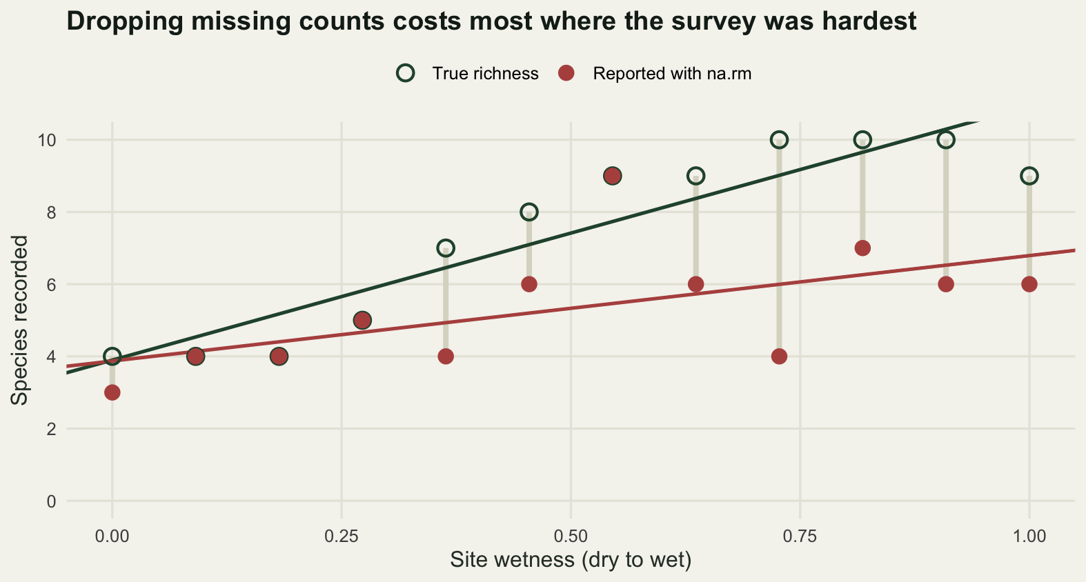
The naive function loses 2.0833 species per site on average, and the average is not the damage. The damage is that the loss is not spread evenly. It is concentrated at the wet end, which is exactly where the ecological signal lives, so the estimated richness gradient is flattened by an amount that depends on survey difficulty rather than on ecology. The true slope is 7.0385 species per unit of wetness and the reported slope is 2.9231, an attenuation of 58.4699 per cent. Of the 66 site pairs, 12.1212 per cent come out strictly the wrong way round, and the rank correlation between true and reported richness drops to 0.6408.
The test is one line, and it is a statement about ecology rather than about code: a site where a species was not counted does not have a known richness. The flagged function passes it, the naive one fails it, and the failing check is named in the report. What the flagged function then forces on you is the real work, which is deciding what to do about the 10 sites whose richness is now NA. That decision belongs in the open, not inside a default argument.
The second bug: per cent where a fraction was expected
Forty quadrats, six species, per-species cover recorded in the field as a percentage. The reading function returns percentages, faithfully. The analysis was written by someone who assumed fractions, and nothing in R objects, because 45 and 0.45 are both plausible cover values until you add them up.
set.seed(41)
n_quad <- 40
n_cov  <- 6
wts <- matrix(rgamma(n_quad * n_cov, shape = 0.9), n_quad, n_cov)
tot_cover <- runif(n_quad, 0.35, 0.92)
cover_frac <- wts / rowSums(wts) * tot_cover
cover_pct  <- 100 * cover_frac
sla <- c(9.5, 14.2, 21.8, 12.4, 27.1, 17.6)
mass_per_cover <- c(480, 260, 150, 330, 110, 200)

bare_ground <- function(cov) pmax(0, 1 - rowSums(cov))
cwm_sla     <- function(cov) rowSums(cov * rep(sla, each = nrow(cov))) / rowSums(cov)
standing_biomass <- function(cov) rowSums(cov * rep(mass_per_cover, each = nrow(cov)))

right <- list(bare = bare_ground(cover_frac), cwm = cwm_sla(cover_frac),
              mass = standing_biomass(cover_frac))
wrong <- list(bare = bare_ground(cover_pct), cwm = cwm_sla(cover_pct),
              mass = standing_biomass(cover_pct))

rel_err <- function(a, b) 100 * max(abs(a - b) / pmax(abs(b), 1e-12))
round(c(quadrats = n_quad,
        true_mean_bare_ground = mean(right$bare),
        reported_mean_bare_ground = mean(wrong$bare),
        quadrats_reported_as_fully_covered = sum(wrong$bare == 0),
        cwm_max_error_percent = rel_err(wrong$cwm, right$cwm),
        biomass_max_error_percent = rel_err(wrong$mass, right$mass)), 4)
quadrats true_mean_bare_ground
40.0000 0.3861
reported_mean_bare_ground quadrats_reported_as_fully_covered
0.0000 40.0000
cwm_max_error_percent biomass_max_error_percent
0.0000 9900.0000 unit_run <- run_new()
unit_run <- expect(unit_run, "cover values are fractions between zero and one",
all(cover_pct >= 0 & cover_pct <= 1))
unit_run <- expect(unit_run, "quadrat cover totals do not exceed one",
all(rowSums(cover_pct) <= 1))
unit_run <- expect(unit_run, "the same two checks on the fractions",
all(cover_frac >= 0 & cover_frac <= 1) &&
all(rowSums(cover_frac) <= 1))
report(unit_run, "units")units : 1 of 3 checks passed | failed: cover values are fractions between zero and one; quadrat cover totals do not exceed oneunit_lab <- c("Community weighted\nmean of leaf area",
"Standing biomass\n(grams per quadrat)",
"Bare ground\n(fraction)")
unit_df <- data.frame(
correct = c(right$cwm, right$mass, right$bare),
reported = c(wrong$cwm, wrong$mass, wrong$bare),
panel = factor(rep(unit_lab, each = n_quad), levels = unit_lab))
span <- do.call(rbind, lapply(unit_lab, function(k) {
z <- unit_df[unit_df$panel == k, c("correct", "reported")]
data.frame(v = range(c(0, unlist(z))), panel = factor(k, levels = unit_lab))
}))
ggplot(unit_df, aes(correct, reported)) +
geom_blank(data = span, aes(v, v)) +
geom_abline(slope = 1, intercept = 0, linetype = 2, colour = te_pal$sage,
linewidth = 0.8) +
geom_point(colour = te_pal$clay, size = 2.2, alpha = 0.85) +
facet_wrap(~panel, scales = "free") +
labs(x = "Value computed from cover fractions",
y = "Value reported from percentages",
title = "One unit error, three completely different consequences") +
theme_te() +
theme(strip.text = element_text(colour = te_pal$ink, face = "bold", size = 9))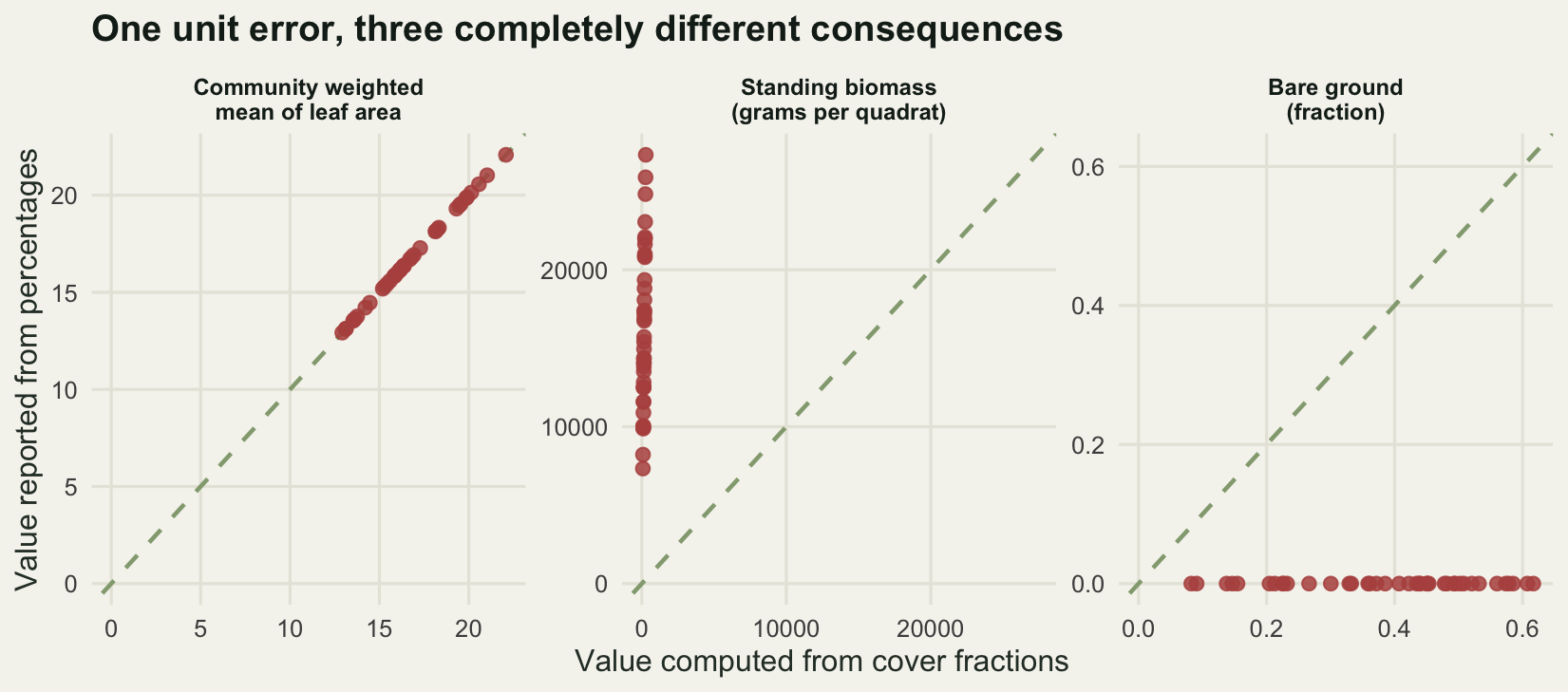
The community weighted mean of specific leaf area is correct. Not approximately correct: the largest relative error across the 40 quadrats is 0 per cent, because a cover-weighted mean divides by the total cover and the scale cancels exactly. Standing biomass is out by 9900 per cent, a factor of one hundred, which is the error you would expect. Bare ground is the interesting one. The true mean bare ground fraction is 0.3861, and the reported mean is 0, in all 40 of the 40 quadrats, because 1 - rowSums(cover) is a large negative number and the defensive pmax(0, ...) turns it into a clean, plausible, entirely wrong zero.
Three checks, each one line. The range check on the values fails, the total-cover check fails, and the same two checks pass on the fractions. That is the whole cost of catching this. Which reported number could have raised the alarm and which could not is the thing to stare at: the community weighted mean, the one that was right to the last digit, is invariant to the bug and therefore could never have warned anybody. Correct output is not evidence of correct code.
Which kind of test earns its lines
Two bugs, two tests, two catches. That proves nothing about which tests to write in general, because both tests were written after the bug was known. The honest way to score a test suite is to break the code on purpose and see what the suite notices. In software engineering that is called mutation testing: make a small edit to a working function, run the tests, record whether they fail, and treat a mutant the tests do not notice as a bug they would also not notice.
The function under test does the standard per-site summary: density per unit of effort, observed richness, the bias-corrected Chao1 estimator of richness, and Shannon diversity. It is held as text so that edits can be made to it programmatically. Note the explicit na.rm = FALSE, which is the fix from the previous section written into the code: a site with an uncounted species gets a row of NA rather than a plausible underestimate.
ref_src <- c(
  "site_stats <- function(counts, effort) {",
  "  ns <- nrow(counts)",
  "  out <- matrix(NA_real_, ns, 4)",
  "  for (i in seq_len(ns)) {",
  "    x <- counts[i, ]",
  "    n <- sum(x, na.rm = FALSE)",
  "    s <- sum(x > 0)",
  "    f1 <- sum(x == 1)",
  "    f2 <- sum(x == 2)",
  "    chao <- s + f1 * (f1 - 1) / (2 * (f2 + 1))",
  "    p <- x[x > 0] / n",
  "    h <- -sum(p * log(p))",
  "    out[i, ] <- c(n / effort[i], s, chao, h)",
  "  }",
  "  colnames(out) <- c('density', 'richness', 'chao1', 'shannon')",
  "  out",
  "}")
ref_txt <- paste(ref_src, collapse = "\n")

compile_fun <- function(txt) {
  env <- new.env(parent = globalenv())
  eval(parse(text = txt), envir = env)
  get("site_stats", envir = env)
}
site_stats <- compile_fun(ref_txt)
stat_names <- c("density", "richness", "chao1", "shannon")

c(target_lines = length(ref_src))
target_lines
17 print(round(site_stats(true_counts, effort), 4)) density richness chao1 shannon
[1,] 7.2368 4 4.5 1.0336
[2,] 12.7517 4 4.0 1.0597
[3,] 8.7500 4 4.5 1.2770
[4,] 29.2683 5 5.0 1.4447
[5,] 40.9091 7 7.0 1.7796
[6,] 21.1268 8 8.0 1.8957
[7,] 28.4615 9 10.0 2.0229
[8,] 28.2051 9 10.0 2.0128
[9,] 51.9231 10 10.0 2.0988
[10,] 56.8966 10 10.0 2.2229
[11,] 66.6667 10 10.0 2.1634
[12,] 68.6747 9 9.0 2.1257The mutation operators are pairs of strings: what to look for, and what to put in its place. Each occurrence of each pattern gives one mutant, so a pattern that appears twice yields two. The families follow the mistakes that actually happen: a boundary moved from strict to non-strict, a constant nudged by one, a division written as a multiplication, a sign flipped, an index shifted by one, an aggregate swapped, a missing data argument flipped, a variable name mistyped for a similar one, and a structural slip such as a swapped pair of columns.
ops <- data.frame(rbind(
  c("relational", "x > 0", "x >= 0"),
  c("constant", "x > 0", "x > 1"),
  c("constant", "== 1", "== 2"),
  c("constant", "== 2", "== 1"),
  c("relational", "sum(x == 2)", "sum(x >= 2)"),
  c("relational", "sum(x == 1)", "sum(x <= 1)"),
  c("sign", "s + f1", "s - f1"),
  c("sign", "f1 - 1", "f1 + 1"),
  c("sign", "f2 + 1", "f2 - 1"),
  c("sign", "-sum(p * log(p))", "sum(p * log(p))"),
  c("constant", "2 * (f2 + 1)", "(f2 + 1)"),
  c("arithmetic", "chao <- s + ", "chao <- s * "),
  c("arithmetic", "] / n", "] * n"),
  c("arithmetic", "n / effort[i]", "n * effort[i]"),
  c("arithmetic", "p * log(p)", "p + log(p)"),
  c("arithmetic", "sum(p * log(p))", "sum(p) * log(p)"),
  c("arithmetic", "log(p)", "log2(p)"),
  c("index shift", "seq_len(ns)", "seq_len(ns - 1)"),
  c("index shift", "seq_len(ns)", "seq_len(ns + 1)"),
  c("index shift", "counts[i, ]", "counts[i - 1, ]"),
  c("index shift", "counts[i, ]", "counts[i + 1, ]"),
  c("index shift", "x[x > 0] / n", "x[x > 0][-1] / n"),
  c("aggregate", "sum(x > 0)", "mean(x > 0)"),
  c("aggregate", "sum(x, na.rm = FALSE)", "mean(x, na.rm = FALSE)"),
  c("missing data", "na.rm = FALSE", "na.rm = TRUE"),
  c("variable swap", "f1 * (f1 - 1)", "f1 * (f2 - 1)"),
  c("structure", "nrow(counts)", "ncol(counts)"),
  c("structure", "matrix(NA_real_, ns, 4)", "matrix(NA_real_, 4, ns)"),
  c("structure", "c(n / effort[i], s, chao, h)", "c(n / effort[i], chao, s, h)"),
  c("structure", "colnames(out) <-", "rownames(out) <-")),
  stringsAsFactors = FALSE)
names(ops) <- c("family", "from", "to")

mutate_at <- function(txt, from, to, k) {
  g <- gregexpr(from, txt, fixed = TRUE)[[1]]
  st <- g[k]
  en <- st + attr(g, "match.length")[k] - 1
  paste0(substr(txt, 1, st - 1), to, substr(txt, en + 1, nchar(txt)))
}

mut <- do.call(rbind, lapply(seq_len(nrow(ops)), function(r) {
  g <- gregexpr(ops$from[r], ref_txt, fixed = TRUE)[[1]]
  if (g[1] == -1) return(NULL)
  data.frame(family = ops$family[r], op = paste(ops$from[r], "to", ops$to[r]),
             site = seq_along(g),
             src = sapply(seq_along(g), function(k)
               mutate_at(ref_txt, ops$from[r], ops$to[r], k)),
             stringsAsFactors = FALSE)
}))
mut <- mut[!duplicated(mut$src), ]
rownames(mut) <- NULL
n_mut <- nrow(mut)
c(operators = nrow(ops), mutants = n_mut)
operators mutants
30 32 print(table(mut$family))
    aggregate    arithmetic      constant   index shift  missing data
            2             6             5             5             1
   relational          sign     structure variable swap
            4             4             4             1
Before a mutant can be scored it has to be classified. Some stop the function outright, and those are killed by anything at all, including simply running the analysis once. Some produce output that no input can distinguish from the reference, and counting those against a test suite would be dishonest. Real equivalence is undecidable, so the proxy used here is empirical: a battery of 300 random count matrices, of varying dimensions, with zeros, singletons, doubletons and missing cells, is pushed through the reference and through every mutant, and a mutant whose output never differs is set aside.
set.seed(907)
n_batt <- 300
battery <- lapply(seq_len(n_batt), function(b) {
  ns <- sample(3:8, 1)
  sp <- sample(3:9, 1)
  cm <- matrix(rpois(ns * sp, sample(c(0.6, 1.4, 3.5), 1)), ns, sp)
  if (runif(1) < 0.3) cm[sample(length(cm), max(1, round(0.12 * length(cm))))] <- NA
  list(counts = cm, effort = round(runif(ns, 0.5, 2), 2))
})

safe_out <- function(fun, case) {
  tryCatch(fun(case$counts, case$effort),
           error = function(e) "stopped", warning = function(w) "stopped")
}
same_out <- function(a, b) {
  if (is.character(a) || is.character(b)) return(identical(a, b))
  if (!identical(dim(a), dim(b)) || !identical(dimnames(a), dimnames(b))) return(FALSE)
  na_a <- is.na(a); na_b <- is.na(b)
  if (!identical(na_a, na_b)) return(FALSE)
  all(abs(a[!na_a] - b[!na_b]) <= 1e-9)
}

ref_battery <- lapply(battery, function(cs) safe_out(site_stats, cs))
mut_funs <- lapply(mut$src, function(s)
  tryCatch(compile_fun(s), error = function(e) NULL))

mut$distinguished <- sapply(seq_len(n_mut), function(m) {
  if (is.null(mut_funs[[m]])) return(TRUE)
  any(!mapply(same_out, lapply(battery, function(cs) safe_out(mut_funs[[m]], cs)),
              ref_battery))
})
mut$stops_everywhere <- sapply(seq_len(n_mut), function(m) {
  if (is.null(mut_funs[[m]])) return(TRUE)
  all(sapply(battery, function(cs)
    identical(safe_out(mut_funs[[m]], cs), "stopped")))
})

round(c(battery_cases = n_batt,
        cases_with_missing_cells = sum(sapply(battery, function(cs)
          anyNA(cs$counts))),
        mutants = n_mut,
        distinguished = sum(mut$distinguished),
        not_distinguished = sum(!mut$distinguished),
        stop_on_every_input = sum(mut$stops_everywhere)), 4)
battery_cases cases_with_missing_cells mutants
300 95 32
distinguished not_distinguished stop_on_every_input
32 0 2 Nothing had to be set aside. All 32 mutants differ from the reference on at least one of the 300 inputs, so every one of them is in principle killable, and 2 of them stop on every single input, which makes them the cheapest kind of bug there is to find.
Now the three suites. The first checks types and shapes and nothing else: is the result a numeric matrix, has it one row per site and the four expected column names, is anything missing or infinite, are richness and density non-negative. The second is a golden test: three small sites worked out on paper, with R used only as a calculator for the logarithms, compared against what the function returns. The third states properties any correct diversity summary must have, without ever saying what the answer is. Species order does not matter; doubling every count leaves richness and diversity alone; halving the effort doubles the density; adding a species that was never seen changes nothing; diversity cannot exceed the log of richness, and an even community sits exactly on that bound; a single-species community has zero diversity; Chao1 is at least the observed richness.
The type and invariant suites take their data as an argument, because later on it matters that the same assertions can be pointed at a different data set. The golden test cannot be moved that way without redoing the arithmetic by hand.
cnt_main <- true_counts
eff_main <- effort
perm_id  <- c(4, 9, 1, 7, 2, 10, 5, 3, 8, 6)

cnt_known <- rbind(c(5, 5, 0, 0), c(8, 1, 1, 0), c(2, 2, 2, 2))
eff_known <- c(1, 2, 4)
known <- rbind(c(10, 2, 2, log(2)),
               c(5, 3, 4, -(0.8 * log(0.8) + 0.2 * log(0.1))),
               c(2, 4, 4, log(4)))
cnt_even  <- rbind(c(3, 3, 3, 3), c(5, 5, 5, 5))
cnt_mono  <- rbind(c(7, 0, 0, 0), c(0, 0, 4, 0))
eff_small <- c(1, 1)

make_type <- function(cnt, eff) function(fun) {
  run <- run_new()
  out <- fun(cnt, eff)
  run <- expect(run, "a numeric matrix", is.matrix(out) && is.numeric(out))
  run <- expect(run, "one row per site", nrow(out) == nrow(cnt))
  run <- expect(run, "four named columns", identical(colnames(out), stat_names))
  run <- expect(run, "nothing missing", !any(is.na(out)))
  run <- expect(run, "everything finite", all(is.finite(out)))
  run <- expect(run, "richness and density not negative",
                all(out[, "richness"] >= 0) && all(out[, "density"] >= 0))
  run
}

suite_known <- function(fun) {
  run <- run_new()
  out <- fun(cnt_known, eff_known)
  run <- expect(run, "site A by hand", near(as.numeric(out[1, ]), known[1, ]))
  run <- expect(run, "site B by hand", near(as.numeric(out[2, ]), known[2, ]))
  run <- expect(run, "site C by hand", near(as.numeric(out[3, ]), known[3, ]))
  run
}

make_invariant <- function(cnt, eff) function(fun) {
  run <- run_new()
  bs <- fun(cnt, eff)
  run <- expect(run, "species order is irrelevant",
                near(as.numeric(fun(cnt[, perm_id], eff)), as.numeric(bs)))
  run <- expect(run, "doubling counts leaves richness and diversity alone",
                near(as.numeric(fun(2 * cnt, eff)[, c("richness", "shannon")]),
                     as.numeric(bs[, c("richness", "shannon")])))
  run <- expect(run, "halving effort doubles density",
                near(as.numeric(fun(cnt, eff / 2)[, "density"]),
                     2 * as.numeric(bs[, "density"])))
  run <- expect(run, "an unseen species changes nothing",
                near(as.numeric(fun(cbind(cnt, 0), eff)), as.numeric(bs)))
  run <- expect(run, "diversity below the log of richness",
                all(bs[, "shannon"] <= log(bs[, "richness"]) + 1e-8))
  run <- expect(run, "an even community sits on the bound",
                near(as.numeric(fun(cnt_even, eff_small)[, "shannon"]),
                     log(as.numeric(fun(cnt_even, eff_small)[, "richness"]))))
  run <- expect(run, "one species means zero diversity",
                near(as.numeric(fun(cnt_mono, eff_small)[, "shannon"]), c(0, 0)))
  run <- expect(run, "chao1 at least richness",
                all(bs[, "chao1"] >= bs[, "richness"]))
  run
}

suites <- list(Types = make_type(cnt_main, eff_main),
               `Known answer` = suite_known,
               Invariants = make_invariant(cnt_main, eff_main))
for (nm in names(suites)) report(suites[[nm]](site_stats), nm)
Types : 6 of 6 checks passed
Known answer : 3 of 3 checks passed
Invariants : 8 of 8 checks passedsuite_catches <- function(suite, fun) {
if (is.null(fun)) return(TRUE)
r <- tryCatch(suite(fun), error = function(e) NULL, warning = function(w) NULL)
if (is.null(r)) return(TRUE)
any(!r$passed)
}
suite_lines <- sapply(suites, function(s) length(deparse(s)))
suite_checks <- sapply(suites, function(s) nrow(s(site_stats)))
print(rbind(lines = suite_lines, checks = suite_checks)) Types Known answer Invariants
lines 15 12 24
checks 6 3 8caught <- sapply(suites, function(s)
sapply(seq_len(n_mut), function(m) suite_catches(s, mut_funs[[m]])))
colnames(caught) <- names(suites)
keep <- mut$distinguished
caught_any <- apply(caught[keep, ], 1, any)
kill_rate <- 100 * colMeans(caught[keep, ])
per_line <- colSums(caught[keep, ]) / suite_lines
print(round(rbind(mutants_caught = colSums(caught[keep, ]),
kill_rate_percent = kill_rate,
lines_of_test_code = suite_lines,
caught_per_line = per_line), 4)) Types Known answer Invariants
mutants_caught 9.000 31.0000 26.0000
kill_rate_percent 28.125 96.8750 81.2500
lines_of_test_code 15.000 12.0000 24.0000
caught_per_line 0.600 2.5833 1.0833round(c(distinguishable = sum(keep),
caught_by_all_three_together = sum(caught_any),
combined_kill_rate_percent = 100 * mean(caught_any),
total_lines_all_three = sum(suite_lines),
missed_by_everything = sum(!caught_any)), 4) distinguishable caught_by_all_three_together
32.000 31.000
combined_kill_rate_percent total_lines_all_three
96.875 51.000
missed_by_everything
1.000 print(mut$op[keep][!caught_any])[1] "na.rm = FALSE to na.rm = TRUE"kill_df <- data.frame(
suite = factor(rep(names(suites), 2), levels = names(suites)),
value = c(kill_rate, per_line),
panel = factor(rep(c("Mutants caught (per cent)",
"Mutants caught per line of test code"),
each = length(suites)),
levels = c("Mutants caught (per cent)",
"Mutants caught per line of test code")))
ggplot(kill_df, aes(suite, value, fill = suite)) +
geom_col(width = 0.62, show.legend = FALSE) +
geom_text(aes(label = sprintf("%.2f", value)), vjust = -0.45, size = 3.4,
colour = te_pal$ink) +
facet_wrap(~panel, scales = "free_y") +
scale_fill_manual(values = c(te_pal$sage, te_pal$gold, te_pal$forest)) +
scale_y_continuous(expand = expansion(mult = c(0, 0.16))) +
labs(x = NULL, y = NULL,
title = "The hand-worked answer is the cheapest test and the sharpest one") +
theme_te() +
theme(strip.text = element_text(colour = te_pal$ink, face = "bold", size = 9))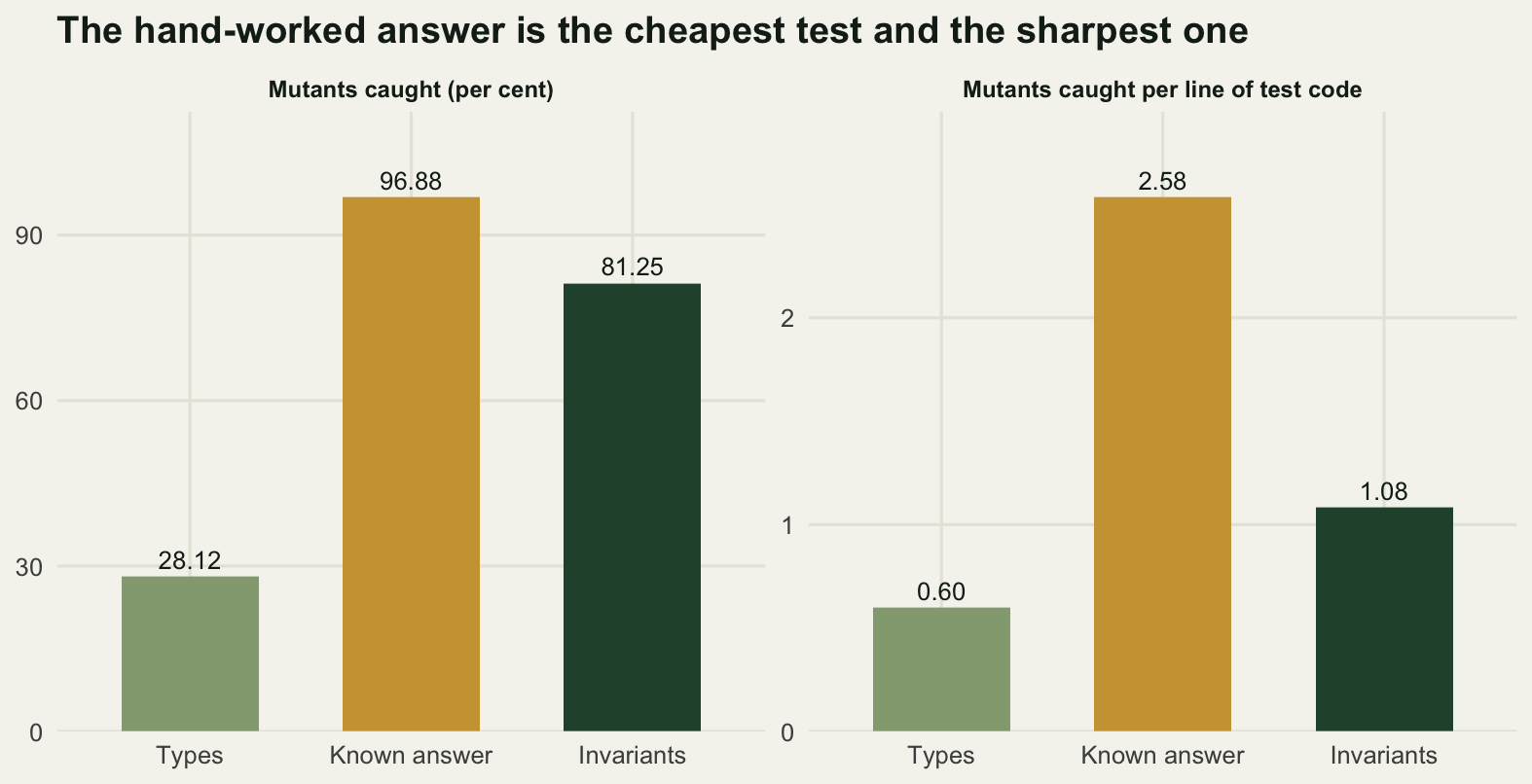
What survives, and what it does to the result
A kill rate is only half the story. The other half is what an undetected edit does to the answer, because a mutant that changes the fourth decimal of Chao1 is not the same problem as one that reorders the sites. Each mutant is put through the twelve-site analysis and its damage measured the same way as in the missing data section: the percentage of the 66 site pairs whose diversity ordering it reverses, with mutants that stop, return missing values or return a table of the wrong shape placed at 100.
ref_shannon <- site_stats(cnt_main, eff_main)[, "shannon"]
damage_of <- function(fun) {
  if (is.null(fun)) return(100)
  out <- tryCatch(fun(cnt_main, eff_main),
                  error = function(e) NULL, warning = function(w) NULL)
  if (is.null(out) || !is.matrix(out)) return(100)
  if (!"shannon" %in% colnames(out) || nrow(out) != n_site) return(100)
  sh <- out[, "shannon"]
  if (anyNA(sh)) return(100)
  pair_flip(ref_shannon, sh)
}
mut$damage <- sapply(mut_funs, damage_of)
mut$caught_any <- apply(caught, 1, any)
mut$n_suites <- rowSums(caught)

surv <- keep & !mut$caught_any
round(c(survivors = sum(surv),
        mutants_that_run_and_leave_the_ranking_alone = sum(mut$damage[keep] == 0),
        mutants_that_reverse_at_least_one_pair = sum(mut$damage[keep] > 0 &
                                                       mut$damage[keep] < 100),
        mutants_that_stop_or_return_missing = sum(mut$damage[keep] == 100),
        worst_damage_percent = max(mut$damage[keep & mut$damage < 100]),
        caught_by_all_three = sum(mut$n_suites[keep] == 3),
        caught_by_exactly_two = sum(mut$n_suites[keep] == 2),
        caught_by_exactly_one = sum(mut$n_suites[keep] == 1)), 4)
survivors
1.0000
mutants_that_run_and_leave_the_ranking_alone
18.0000
mutants_that_reverse_at_least_one_pair
5.0000
mutants_that_stop_or_return_missing
9.0000
worst_damage_percent
92.4242
caught_by_all_three
9.0000
caught_by_exactly_two
17.0000
caught_by_exactly_one
5.0000 part <- keep & mut$damage > 0 & mut$damage < 100
print(data.frame(op = mut$op[part], family = mut$family[part],
damage_percent = round(mut$damage[part], 4),
suites_catching = mut$n_suites[part])[order(-mut$damage[part]), ]) op family damage_percent suites_catching
2 ] / n to ] * n arithmetic 92.4242 2
3 p * log(p) to p + log(p) arithmetic 13.6364 2
4 counts[i, ] to counts[i - 1, ] index shift 6.0606 2
1 x > 0 to x > 1 constant 3.0303 2
5 x[x > 0] / n to x[x > 0][-1] / n index shift 1.5152 2print(data.frame(op = mut$op[surv], family = mut$family[surv],
damage_on_complete_data = round(mut$damage[surv], 2))) op family damage_on_complete_data
1 na.rm = FALSE to na.rm = TRUE missing data 0The one survivor is the na.rm flip, and the reason it survives is the most useful thing in this post. Every input in all three suites is complete. A mutant that changes only what happens to missing values cannot be caught by a test that never supplies one, however clever the assertion. On complete data it does no damage at all, which is why it slips through. On the observed matrix from the first section it does the damage the first section was about. The kill rate is a property of the test corpus at least as much as of the assertions.
Three further measurements make that concrete. The first adds a single case, the observed count matrix with its gaps, and asks only that the result match the reference. The second points the type and invariant suites at 20 different randomly generated count matrices, leaving their assertions untouched, and records how the kill rate moves. The third runs the survivor on the observed data and compares it against the truth.
na_case <- list(counts = obs_counts, effort = eff_main)
extra_check <- function(fun) {
  if (is.null(fun)) return(TRUE)
  out <- tryCatch(fun(na_case$counts, na_case$effort),
                  error = function(e) NULL, warning = function(w) NULL)
  if (is.null(out) || !is.matrix(out)) return(TRUE)
  !same_out(out, site_stats(na_case$counts, na_case$effort))
}
with_na <- caught_any | sapply(mut_funs[keep], extra_check)
round(c(combined_kill_rate_percent = 100 * mean(caught_any),
        kill_rate_with_one_extra_case_percent = 100 * mean(with_na),
        survivors_after_the_extra_case = sum(!with_na)), 4)
combined_kill_rate_percent kill_rate_with_one_extra_case_percent
96.875 100.000
survivors_after_the_extra_case
0.000 surv_out <- mut_funs[[which(surv)]](obs_counts, eff_main)
truth_out <- site_stats(true_counts, eff_main)
round(c(survivor_mean_density_error_percent =
100 * mean(abs(surv_out[, "density"] - truth_out[, "density"]) /
truth_out[, "density"]),
survivor_worst_density_error_percent =
100 * max(abs(surv_out[, "density"] - truth_out[, "density"]) /
truth_out[, "density"]),
survivor_density_pairs_reversed_percent =
pair_flip(truth_out[, "density"], surv_out[, "density"]),
survivor_sites_left_missing = sum(is.na(surv_out[, "richness"]))), 4) survivor_mean_density_error_percent survivor_worst_density_error_percent
22.7366 58.3333
survivor_density_pairs_reversed_percent survivor_sites_left_missing
10.6061 10.0000 set.seed(3105)
n_corp <- 20
alt_rate <- sapply(seq_len(n_corp), function(k) {
cm <- matrix(rpois(n_site * n_spec, sample(c(0.7, 2, 5), 1)), n_site, n_spec)
ef <- round(runif(n_site, 0.6, 1.8), 2)
sapply(list(make_type(cm, ef), make_invariant(cm, ef)), function(s)
mean(sapply(mut_funs[keep], function(f) suite_catches(s, f))))
})
rownames(alt_rate) <- c("Types", "Invariants")
round(rbind(corpora = c(n_corp, n_corp),
lowest_percent = 100 * apply(alt_rate, 1, min),
median_percent = 100 * apply(alt_rate, 1, median),
highest_percent = 100 * apply(alt_rate, 1, max),
on_the_field_data_percent = kill_rate[c("Types", "Invariants")]), 4) Types Invariants
corpora 20.000 20.0000
lowest_percent 25.000 65.6250
median_percent 28.125 79.6875
highest_percent 28.125 81.2500
on_the_field_data_percent 28.125 81.2500dam_df <- mut[keep, ]
fam_order <- names(sort(tapply(dam_df$damage, dam_df$family, mean)))
dam_df$family <- factor(dam_df$family, levels = fam_order)
dam_df$cover <- factor(dam_df$n_suites, levels = 0:3,
labels = c("none", "one", "two", "all three"))
ggplot(dam_df, aes(damage, family, fill = cover)) +
geom_point(size = 3.6, shape = 21, colour = te_pal$ink, stroke = 0.7,
position = position_nudge(y = ave(dam_df$damage, dam_df$family,
dam_df$damage,
FUN = function(z)
0.17 * (seq_along(z) - 1)))) +
scale_fill_manual(values = c(te_pal$paper, te_pal$gold, te_pal$sage,
te_pal$forest),
name = "Suites that catch it", drop = FALSE) +
scale_x_continuous(limits = c(-4, 104)) +
labs(x = "Site pairs whose diversity ranking is reversed (per cent)", y = NULL,
title = "Most small edits either stop the run or leave the ranking alone") +
theme_te() +
theme(legend.position = "top")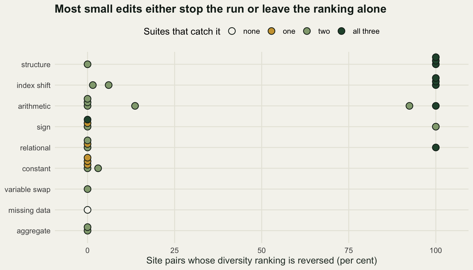
The three suites together, 51 lines of test code, catch 96.875 per cent of the 32 mutants. Adding that one extra input with gaps in it takes the combined rate to 100 per cent and leaves nothing alive. One case, no new assertion, and the only survivor dies.
The survivor is not idle while nobody looks at it. Run on the observed counts, it underestimates density at most of the sites, by 22.7366 per cent averaged over all twelve and 58.3333 per cent at the worst site, and it reverses 10.6061 per cent of the site pairs ranked by density. The only outward sign is that the richness column comes back missing at 10 sites, which is the kind of thing a tired analyst fixes with another na.rm rather than investigates.
The per-suite figures are not the ordering I expected before running this. The golden test catches 96.875 per cent from 12 lines, the invariants 81.25 per cent from 24 lines, and the type suite 28.125 per cent from 15 lines. Per line of test code that is 2.58, 1.08 and 0.60 mutants, so the hand-worked answer wins on both measures and wins the per-line comparison by more than a factor of two. The reason is not subtle once you see it: three sites worked out on paper pin down twelve numbers at once, and almost any edit to the function moves at least one of them. Property tests are weaker per assertion because each property constrains only a direction, not a value.
The corpus measurement is where the invariants earn their place. Pointed at 20 different random count matrices, the invariant suite catches between 65.625 and 81.25 per cent of the mutants, with a median of 79.6875, and the type suite between 25 and 28.125 per cent. Neither collapses. The golden test has no such range because it cannot be pointed anywhere: its three sites were worked out by hand, and a new data set means a new hand computation. A suite of properties keeps testing when the data change, which is what you want from the checks that run on every new season of fieldwork, and a golden test is the sharpest instrument you have for the data it was written against.
The damage figure adds the part a kill rate cannot show. Of the 32 mutants, 18 leave the diversity ranking of the twelve sites exactly as it was, 9 sit at one hundred per cent on the damage scale, and 5 keep running and reorder part of the ranking. Most of the 9 stop the function or fill it with missing values; one returns a table of the wrong shape, and one is the sign flip on the Shannon sum, which runs without error and reverses every pair. That sign flip and the 5 partial reorderings are the dangerous ones, and they are not where the eye goes: a flipped sign, two arithmetic slips, two index shifts and one moved constant. The worst of the 5 turns a division into a multiplication and reverses 92.4242 per cent of the pairs, which is a different site ranking rather than a damaged one. Every one of the 5 was caught by exactly two of the three suites, and the redundancy elsewhere is not evenly spread: 9 of the 32 mutants are caught by all three suites and 5 by only one.
The honest limit
Mutation score measures whether a test suite notices changes to the code. It does not measure whether the code is right. That distinction is not academic, because the most expensive failure in this post is exactly of the kind the score cannot see.
Take the naive version from the first section, the one that drops missing counts throughout, and treat it as the reference. Build a golden test from its own output, the way a hurried analyst does when the function is already written and a test is being added to satisfy a reviewer.
naive_txt <- paste(c(
  "site_stats <- function(counts, effort) {",
  "  ns <- nrow(counts)",
  "  out <- matrix(NA_real_, ns, 4)",
  "  for (i in seq_len(ns)) {",
  "    x <- counts[i, ]",
  "    x <- x[!is.na(x)]",
  "    n <- sum(x, na.rm = TRUE)",
  "    s <- sum(x > 0)",
  "    f1 <- sum(x == 1)",
  "    f2 <- sum(x == 2)",
  "    chao <- s + f1 * (f1 - 1) / (2 * (f2 + 1))",
  "    p <- x[x > 0] / n",
  "    h <- -sum(p * log(p))",
  "    out[i, ] <- c(n / effort[i], s, chao, h)",
  "  }",
  "  colnames(out) <- c('density', 'richness', 'chao1', 'shannon')",
  "  out",
  "}"), collapse = "\n")
naive_fun <- compile_fun(naive_txt)
blessed <- naive_fun(obs_counts, eff_main)

suite_blessed <- function(fun) {
  run <- run_new()
  out <- fun(obs_counts, eff_main)
  run <- expect(run, "matches the recorded output",
                near(as.numeric(out), as.numeric(blessed)))
  run
}
blessed_kill <- mean(sapply(mut_funs[keep], function(f)
  suite_catches(suite_blessed, f)))

round(c(blessed_suite_lines = length(deparse(suite_blessed)),
        blessed_kill_rate_percent = 100 * blessed_kill,
        blessed_also_rejects_the_corrected_function =
          suite_catches(suite_blessed, site_stats),
        blessed_mean_richness = mean(blessed[, "richness"]),
        true_mean_richness = mean(true_rich),
        blessed_slope = coef(lm(blessed[, "richness"] ~ wetness))[2],
        true_slope = slope_true[2],
        blessed_pairs_reversed_percent =
          pair_flip(true_rich, blessed[, "richness"])), 4)
blessed_suite_lines
8.0000
blessed_kill_rate_percent
100.0000
blessed_also_rejects_the_corrected_function
1.0000
blessed_mean_richness
5.3333
true_mean_richness
7.4167
blessed_slope.wetness
2.9231
true_slope.wetness
7.0385
blessed_pairs_reversed_percent
12.1212 That one-assertion suite, 8 lines as R deparses it, kills 100 per cent of the mutants, which beats every suite written with care in the previous section. It is also wrong about the ecology. It reports a mean richness of 5.3333 against a true 7.4167 and a richness gradient of 2.9231 species per unit of wetness against a true 7.0385, and it reverses 12.1212 per cent of the site pairs, because it has written the missing data bug into the specification and then defended it. It fails the corrected function, which it treats as the broken one. A test that says the answer is whatever the code said yesterday is a regression test. Regression tests are worth having, but a high mutation score from a suite like that means only that the code has not changed.
Three further limits are worth stating. The equivalence classification here is empirical: 300 random inputs distinguished all 32 mutants, so nothing had to be set aside, but that is a fact about this battery, not a proof, and true equivalence is undecidable. The mutation operators are a model of what programmers get wrong rather than a sample of real ecological analysis bugs, and the software engineering literature treats mutants as a reasonable but imperfect stand-in for real faults. And nothing here tests the statistics: a suite can be complete and green while the model behind the analysis is the wrong model for the data, which is a different kind of checking altogether.
Where to go next
The cheapest next step is not more tests. It is making the analysis fail loudly at its own boundaries, which is the subject of debugging and defensive R code: stopifnot at the top of a function is a test that travels with the code and runs on real data rather than on three sites made up for the purpose. After that, checking an analysis script takes the whole file rather than one function and asks whether it runs from a clean session, gives the same answer twice, and reports the numbers it actually computed.
If you write more than one analysis with the same helper functions in it, the test suite becomes an argument for putting those functions somewhere shared, which is where turning your code into an R package starts, and the tests/testthat/ layout in the non-executed block above is what it looks like once you get there.
References
Wilson G, Aruliah DA, Brown CT, Chue Hong NP, Davis M, Guy RT, Haddock SHD, Huff KD, Mitchell IM, Plumbley MD, Waugh B, White EP, Wilson P 2014 PLoS Biology 12(1):e1001745 (10.1371/journal.pbio.1001745)
Wilson G, Bryan J, Cranston K, Kitzes J, Nederbragt L, Teal TK 2017 PLoS Computational Biology 13(6):e1005510 (10.1371/journal.pcbi.1005510)
Sandve GK, Nekrutenko A, Taylor J, Hovig E 2013 PLoS Computational Biology 9(10):e1003285 (10.1371/journal.pcbi.1003285)
Baker M 2016 Nature 533(7604):452-454 (10.1038/533452a)
Jia Y, Harman M 2011 IEEE Transactions on Software Engineering 37(5):649-678 (10.1109/TSE.2010.62)
Chao A 1984 Scandinavian Journal of Statistics 11(4):265-270 (No DOI)