library(ggplot2)

te_pal <- list(forest = "#275139", green = "#2f8f63", sage = "#93a87f",
               clay = "#b5534e", gold = "#cda23f", line = "#dad9ca",
               ink = "#16241d", paper = "#f5f4ee")

theme_te <- function() {
  theme_minimal(base_size = 12) +
    theme(panel.grid.minor = element_blank(),
          panel.grid.major = element_line(colour = "#e7e6dc"),
          plot.background = element_rect(fill = "#f5f4ee", colour = NA),
          panel.background = element_rect(fill = "#f5f4ee", colour = NA),
          plot.title = element_text(face = "bold", colour = te_pal$ink),
          axis.title = element_text(colour = "#2c3a31"))
}Checking an analysis script
R
reproducibility
model diagnostics
ecology tutorial
ggplot2
Four checks on an R analysis script for ecologists: a clean session run, repeatability under seeds, row order dependence, and reported numbers against output.
Step 42 of the Tidy Ecology course, Part eight: make the result hold up.
A colleague sends you a folder: a script, a data file, and a figure that is already in a manuscript. The script runs. The figure appears. The number in the abstract is in the figure caption. Everything about the folder says that the work is finished, and nothing about it says whether the number in the abstract is the number the script produces today, on your machine, from that data file.
This post runs four checks on one small analysis of pitfall trap data, built here so that the right answer is known throughout. Does the script run from the top in an empty session, does it give the same answer twice, does it survive the rows arriving in a different order, and does the number written in the prose match the number the code prints. Each check ends in a measured quantity: how far the reported effect moves, how much the answer moves between two runs of the same code, how many of the reported numbers change, how many real errors a checker catches and how many false alarms it raises on the way.
The three sibling posts in this cluster attack the same problem from other sides. Testing your analysis code writes assertions that a function has to satisfy. Debugging and defensive R code chases the error that runs to completion and returns the wrong number. Speeding up your analysis code measures where the time goes. This one takes a finished script that nobody suspects and asks what it would take to trust it.
The script under test
Twelve grassland sites, six grazed and six ungrazed, each trapped over five rounds with pitfall traps. Every record carries the site, the treatment, the round, the number of trap nights the trap was open, the beetle catch and the number of morphospecies in the sample. The analysis is the kind that fits on one screen: standardise each catch to a rate per hundred trap nights, drop the samples where the trap was never set, remove the records that were entered twice, average up to the site, weight the sites by trapping effort, and report the percentage difference between the grazed and the ungrazed sites.
The data are simulated so that the truth is available, and three faults are built into them on purpose because they are the faults that field data actually carries. Four samples have zero trap nights because the trap was lost or flooded. Three samples were entered twice, with a different catch the second time, which is what happens when a spreadsheet is merged from two field books. Three samples had eight trap nights transcribed as two, which is the kind of slip that turns a rate into an outlier.
set.seed(20260813)

n_site <- 12
site_id <- sprintf("S%02d", 1:n_site)
grp <- rep(c("grazed", "ungrazed"), each = 6)
rounds <- 5

raw <- expand.grid(round = 1:rounds, site = site_id, stringsAsFactors = FALSE)
raw$treat <- grp[match(raw$site, site_id)]
raw$nights <- sample(c(4, 5, 6, 7, 8, 8, 9, 10, 12), nrow(raw), replace = TRUE)
lam <- ifelse(raw$treat == "grazed", 3.4, 2.3) *
  exp(rnorm(n_site, 0, 0.25))[match(raw$site, site_id)]
raw$beetles <- rpois(nrow(raw), lam * raw$nights)
raw$species <- rpois(nrow(raw), 4 + 0.03 * raw$beetles)
raw <- raw[, c("site", "treat", "round", "nights", "beetles", "species")]

lost <- c(11, 24, 39, 55)
raw$nights[lost] <- 0
raw$beetles[lost] <- 0
raw$species[lost] <- 0

slip <- c(3, 17, 26)
raw$nights[slip] <- 8
raw$beetles[slip] <- rpois(3, lam[slip] * 8)
raw$nights[slip] <- 2

dup <- c(9, 34, 52)
extra <- raw[dup, ]
extra$beetles <- extra$beetles + c(11, -8, 14)
extra$species <- extra$species + c(1, -1, 2)
raw <- rbind(raw, extra)
raw <- raw[order(raw$site, raw$round), ]
rownames(raw) <- NULL
slip_row <- which(raw$nights == 2)

print(head(raw, 6))
site treat round nights beetles species
1 S01 grazed 1 7 45 5
2 S01 grazed 2 10 48 1
3 S01 grazed 3 2 38 6
4 S01 grazed 4 10 39 3
5 S01 grazed 5 9 50 9
6 S02 grazed 1 9 41 2c(sites = n_site, rounds = rounds, records = nrow(raw),
zero_night = sum(raw$nights == 0),
duplicated_records = sum(duplicated(raw[, c("site", "round")])),
transcription_slips = length(slip_row)) sites rounds records zero_night
12 5 63 4
duplicated_records transcription_slips
3 3 The script itself is held as a list of statements so that it can be run from any point rather than only from the top. That is the only artificial thing about it: the statements are exactly the lines an analyst would write, in the order they would write them, and the first one stands in for the line that reads the data file.
script <- list(
  quote(dat <- raw),
  quote(dat$dens <- 100 * dat$beetles / dat$nights),
  quote(keep <- dat[dat$nights >= 1, ]),
  quote(keep <- keep[!duplicated(keep[, c("site", "round")]), ]),
  quote(sites <- unique(keep$site)),
  quote(site_dens <- sapply(sites, function(s) mean(keep$dens[keep$site == s]))),
  quote(site_rich <- sapply(sites, function(s) mean(keep$species[keep$site == s]))),
  quote(site_grp <- sapply(sites, function(s) keep$treat[keep$site == s][1])),
  quote(effort <- sapply(sites, function(s) sum(dat$nights[dat$site == s]))),
  quote(wt <- effort / sum(effort)),
  quote(m_g <- weighted.mean(site_dens[site_grp == "grazed"], wt[site_grp == "grazed"])),
  quote(m_u <- weighted.mean(site_dens[site_grp == "ungrazed"], wt[site_grp == "ungrazed"])),
  quote(effect <- 100 * (m_g - m_u) / m_u),
  quote(zed <- scale(cbind(site_dens, site_rich))),
  quote(grp2 <- cutree(hclust(dist(zed)), k = 2)),
  quote(g1_dens <- mean(site_dens[grp2 == 1]))
)

run_from <- function(e, from) {
  for (i in from:length(script)) eval(script[[i]], e)
  e
}
run_all <- function(d) run_from(list2env(list(raw = d), parent = globalenv()), 1)

e_file <- run_all(raw)
fixed <- raw
fixed$nights[slip_row] <- 8
e_fixed <- run_all(fixed)

c(statements = length(script))
statements
16 round(c(as_the_file_stands = e_file$effect, with_the_slips_repaired = e_fixed$effect), 4) as_the_file_stands with_the_slips_repaired
118.6719 66.5051 round(c(grazed = e_fixed$m_g, ungrazed = e_fixed$m_u), 3) grazed ungrazed
388.241 233.171 Run as it stands, the script reports the grazed sites as 118.6719 per cent above the ungrazed ones. With the three transcription slips repaired, the same script on the same data reports 66.5051 per cent, from a grazed mean of 388.241 beetles per hundred trap nights against 233.171. Both numbers are produced without an error, without a warning, and without anything on screen to separate them. Everything below is about the distance between them and about the several other numbers hiding in the same script.
Check 1: does it run from the top in an empty session?
The analyst who spots the transcription slips has two ways to fix them. One is to edit the data file or add a correction line to the script. The other is to type the correction at the console, which takes four seconds, works immediately, and leaves no trace in the file. After that the workspace and the script disagree about what the data are, and every subsequent run mixes them in a way that depends on where the cursor was.
Selecting a block and running it is the normal way to work in R, and it is not the problem on its own. The problem is that the objects a script creates persist, so re-running from statement seven recomputes statements seven onwards from whatever statements one to six left behind. If nothing has changed outside the script the result is the same as before. If a correction has been typed at the console, the result is a blend of the corrected and the uncorrected analysis, and which blend you get depends on a keystroke.
The check is a sweep: apply the console correction to the workspace copy of the data, then resume the script from each of its statements in turn, and record the number that comes out.
n_warn <- 0
resume <- withCallingHandlers(
  sapply(seq_along(script), function(r) {
    e <- run_all(raw)
    e$dat$nights[slip_row] <- 8
    run_from(e, r)$effect
  }),
  warning = function(w) { n_warn <<- n_warn + 1; invokeRestart("muffleWarning") })
names(resume) <- seq_along(script)
print(round(resume, 4))
1 2 3 4 5 6 7 8
118.6719 66.5051 124.3762 124.3762 124.3762 124.3762 124.3762 124.3762
9 10 11 12 13 14 15 16
124.3762 118.6719 118.6719 118.6719 118.6719 118.6719 118.6719 118.6719 round(c(distinct_answers = length(unique(round(resume, 8))),
lowest = min(resume), highest = max(resume),
spread = diff(range(resume)),
clean_session = e_file$effect,
what_the_analyst_believes = e_fixed$effect), 4) distinct_answers lowest highest
3.0000 66.5051 124.3762
spread clean_session what_the_analyst_believes
57.8711 118.6719 66.5051 c(warnings_raised_by_the_sweep = n_warn)warnings_raised_by_the_sweep
0 rs <- data.frame(statement = seq_along(resume), effect = as.numeric(resume))
ggplot(rs, aes(statement, effect)) +
geom_hline(yintercept = e_file$effect, colour = te_pal$clay,
linetype = "22", linewidth = 0.6) +
geom_hline(yintercept = e_fixed$effect, colour = te_pal$forest, linewidth = 0.6) +
geom_point(colour = te_pal$ink, size = 3) +
scale_x_continuous(breaks = seq(1, 16, by = 3)) +
scale_y_continuous(expand = expansion(mult = 0.12)) +
labs(x = "Statement the analyst resumed from", y = "Reported effect (per cent)",
title = "Where you resume the script decides the number it reports") +
theme_te()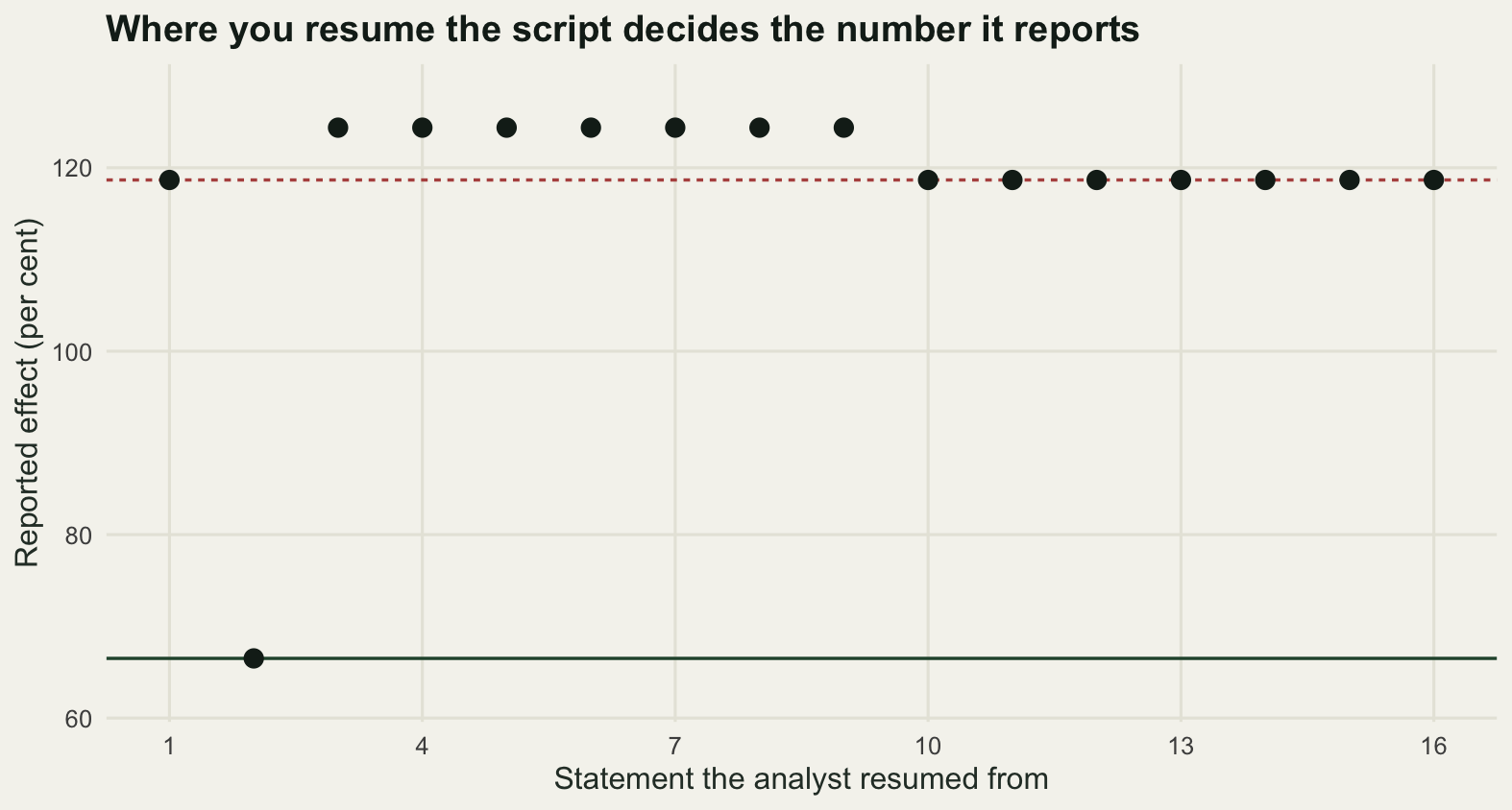
Sixteen resume points give three different answers. Resuming from the top restores the data line and wipes the console correction out, so the script reports 118.6719 per cent: reproducible, and wrong in the sense that the analyst knows the trap nights were mistyped. Resuming from the second statement recomputes everything from the corrected data and gives 66.5051 per cent, which is the number the analyst thinks they have. Resuming from anywhere between the third and the ninth statement gives 124.3762 per cent, which is nobody’s analysis: the density column is stale, computed from the mistyped trap nights, while the effort weights underneath it are recomputed from the corrected ones. Resuming from the tenth statement or later leaves the whole density calculation stale and returns 118.6719 again.
The spread across the sixteen resume points is 57.8711 percentage points on an estimate of about sixty-six, and the whole sweep raised 0 warnings. The highest answer is the interesting one, because it is the only one of the three that no complete run of any version of the script can produce. It exists solely as a residue of the order in which lines were sent to the console, and it is the number that would have gone into the manuscript if the analyst had happened to put the cursor on the filtering line.
Clearing the workspace is half the fix and the smaller half. Deleting every object forces the script to rebuild what it needs, but it only helps if the next run starts at the top, and it does not capture the option settings, the loaded packages or the working directory, which is why the check has to be a fresh process rather than a fresh workspace. Setting up R for ecology covers the settings that make this the default: never restore the workspace at startup, never save it at exit. The check itself is one line in a terminal, and it is worth running before anything leaves the building.
R --vanilla -f analysis.RCheck 2: does it give the same answer twice?
The script above is deterministic. The moment a bootstrap interval or a permutation test is added it stops being deterministic, and the question of whether it gives the same answer twice becomes a question about the random number stream. The analysis here resamples sites within treatment for a percentile interval on the effect, and permutes the treatment labels across sites for a p-value.
sd_v <- e_fixed$site_dens; wt_v <- e_fixed$wt; g_v <- e_fixed$site_grp
obs <- e_fixed$effect
n_boot <- 2000
n_perm <- 999
n_run <- 200

eff_of <- function(ig, iu) {
  b <- nrow(ig)
  ag <- rowSums(matrix(sd_v[ig] * wt_v[ig], nrow = b)) / rowSums(matrix(wt_v[ig], nrow = b))
  au <- rowSums(matrix(sd_v[iu] * wt_v[iu], nrow = b)) / rowSums(matrix(wt_v[iu], nrow = b))
  100 * (ag - au) / au
}
boot_ci <- function(b = n_boot) {
  ig <- which(g_v == "grazed"); iu <- which(g_v == "ungrazed")
  mg <- matrix(sample(ig, b * length(ig), replace = TRUE), nrow = b)
  mu <- matrix(sample(iu, b * length(iu), replace = TRUE), nrow = b)
  unname(quantile(eff_of(mg, mu), c(0.025, 0.975)))
}
perm_p <- function(p = n_perm) {
  st <- replicate(p, {
    gg <- sample(g_v)
    100 * (weighted.mean(sd_v[gg == "grazed"], wt_v[gg == "grazed"]) /
             weighted.mean(sd_v[gg == "ungrazed"], wt_v[gg == "ungrazed"]) - 1)
  })
  (1 + sum(abs(st) >= abs(obs))) / (p + 1)
}

set.seed(20260813)
loose <- t(replicate(n_run, boot_ci()))
loose_p <- replicate(n_run, perm_p())
tight <- t(replicate(50, { set.seed(20260813); boot_ci() }))

c(replicates = n_boot, permutations = n_perm, runs = n_run)
replicates permutations runs
2000 999 200 round(c(upper_mean = mean(loose[, 2]), upper_sd = sd(loose[, 2]),
upper_low = min(loose[, 2]), upper_high = max(loose[, 2]),
lower_sd = sd(loose[, 1]), mean_width = mean(loose[, 2] - loose[, 1])), 4)upper_mean upper_sd upper_low upper_high lower_sd mean_width
96.3032 0.9761 94.2211 99.4999 0.7981 58.8006 round(c(p_mean = mean(loose_p), p_sd = sd(loose_p),
p_low = min(loose_p), p_high = max(loose_p)), 4)p_mean p_sd p_low p_high
0.0031 0.0015 0.0010 0.0080 c(distinct_seeded_intervals = nrow(unique(round(tight, 10))))distinct_seeded_intervals
1 run_a <- function() { set.seed(20260813); ci <- boot_ci(); p <- perm_p(); c(ci, p) }
run_b <- function() { set.seed(20260813); p <- perm_p(); ci <- boot_ci(); c(ci, p) }
ord_a <- run_a(); ord_b <- run_b()
ggplot(data.frame(upper = loose[, 2]), aes(upper)) +
geom_histogram(binwidth = 0.25, fill = te_pal$sage, colour = te_pal$forest,
linewidth = 0.3) +
geom_vline(xintercept = ord_a[2], colour = te_pal$clay, linewidth = 0.9) +
geom_vline(xintercept = ord_b[2], colour = te_pal$ink, linetype = "22", linewidth = 0.7) +
labs(x = "Upper limit of the interval (per cent)", y = "Runs",
title = "An unseeded bootstrap reports a different limit every run") +
theme_te()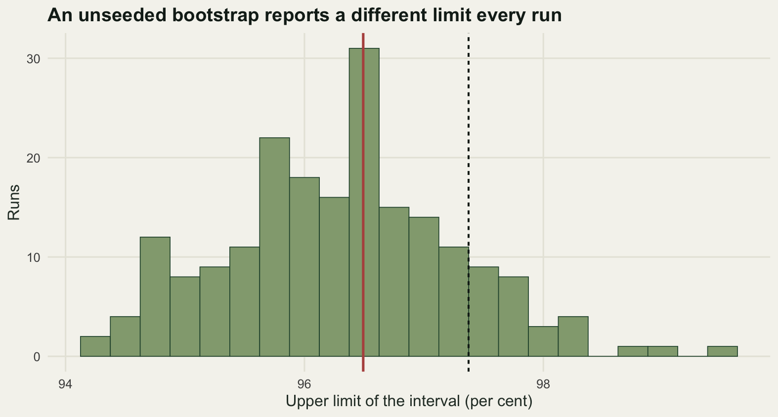
Two hundred runs of the unseeded bootstrap, on data that never changed, put the upper limit anywhere between 94.2211 and 99.4999, with a standard deviation of 0.9761 across runs on a mean interval width of 58.8006. The lower limit wanders by 0.7981. The p-value from the permutation test has a mean of 0.0031 across runs and a range from 0.0010 to 0.0080, so here the same test gives values a factor of eight apart on the same data. Setting the seed inside the run removes all of it: fifty seeded runs produce 1 distinct interval.
That is the well known part. The part that gets missed is that the seed attaches to the stream, not to the calculation, so it only fixes the answer if everything upstream of the calculation also stays put. The next block runs the same two procedures under one seed at the top of the script in the two possible orders, and then displaces the stream by a throwaway draw of increasing size before the bootstrap, which stands for the diagnostic line that gets typed, looked at, and left in.
comp <- rbind(bootstrap_first = ord_a, permutation_first = ord_b)
colnames(comp) <- c("lower", "upper", "p_value")
print(round(comp, 4))
lower upper p_value
bootstrap_first 39.1353 96.4919 0.001
permutation_first 37.9091 97.3739 0.004round(c(upper_shift_from_reordering = ord_b[2] - ord_a[2],
p_shift_from_reordering = ord_b[3] - ord_a[3]), 4)upper_shift_from_reordering p_shift_from_reordering
0.882 0.003 displace <- c(1, 10, 100, 500, 1000, 2000, 4000, 12000)
shifted <- sapply(displace, function(j) {
set.seed(20260813); invisible(runif(j)); boot_ci()[2]
})
names(shifted) <- displace
print(round(shifted - ord_a[2], 4)) 1 10 100 500 1000 2000 4000 12000
0.0000 0.0000 0.0000 -0.0478 0.6668 0.3123 0.3101 -1.1358 reps_of <- function(j) {
set.seed(20260813); if (j > 0) invisible(runif(j))
ig <- which(g_v == "grazed"); iu <- which(g_v == "ungrazed")
eff_of(matrix(sample(ig, n_boot * 6, replace = TRUE), nrow = n_boot),
matrix(sample(iu, n_boot * 6, replace = TRUE), nrow = n_boot))
}
r0 <- reps_of(0); r1 <- reps_of(1)
c(replicates_shared_after_one_throwaway_draw = sum(r0[-1] == r1[-n_boot]))replicates_shared_after_one_throwaway_draw
1999 per_block <- function(swap) {
if (swap) { set.seed(20260814); p <- perm_p(); set.seed(20260813); ci <- boot_ci() }
else { set.seed(20260813); ci <- boot_ci(); set.seed(20260814); p <- perm_p() }
c(ci, p)
}
round(c(largest_difference_with_a_seed_per_block =
max(abs(per_block(TRUE) - per_block(FALSE)))), 6)largest_difference_with_a_seed_per_block
0 With one seed at the top, moving the permutation test above the bootstrap moves the upper limit by 0.8820 and the p-value by 0.0030, from 0.0010 to 0.0040. The edit does not touch the analysis. The bootstrap resamples the same sites with the same weights either way; it just starts from a different point in the stream, and a percentile interval from two thousand draws is a random variable whose spread the histogram above measures. Seeding each stochastic block separately makes the reordering irrelevant, and the largest difference between the two orders drops to exactly zero.
The displacement sweep says something more specific about how much of the stream an edit has to move before the answer moves with it. Throwing away 1, 10 or 100 numbers before the bootstrap leaves the upper limit unchanged to every printed digit. From 500 onwards it moves, and at a displacement of 12000 the limit comes out 1.1358 lower. The reason is in the way the resampling matrix is filled: it takes one long draw and cuts it into replicates, so displacing the stream by one number gives a set of replicates that shares 1999 of its 2000 members with the original. A displacement of the order of the number of replicates replaces the sample outright, and the permutation block, at 999 permutations of 12 site labels, displaces far more than that. The practical reading is not that small edits are safe. It is that the same edit is harmless in one script and consequential in the next, which is why the rule has to be mechanical rather than judged case by case.
There is a second reading of these numbers that matters more than the reproducibility point. The run to run standard deviation of the upper limit, 0.9761, is the Monte Carlo error of the reported statistic, and it is what tells you how many digits of that limit are real.
set.seed(20260813)
sd_big <- sd(replicate(50, boot_ci(4 * n_boot)[2]))
round(c(sd_at_2000 = sd(loose[, 2]), sd_at_8000 = sd_big,
        ratio = sd(loose[, 2]) / sd_big, expected_ratio = 2), 4)
sd_at_2000 sd_at_8000 ratio expected_ratio
0.9761 0.5060 1.9289 2.0000 c(millions_of_replicates_for_two_decimals =
round(n_boot * (sd(loose[, 2]) / 0.005)^2 / 1e6))millions_of_replicates_for_two_decimals
76 Quadrupling the number of resamples divides the run to run standard deviation by 1.9289, against the 2 the square root law predicts. Reporting the upper limit as 96.4919, as the seeded run invites you to, claims every printed digit on a quantity whose own sampling noise is of the order of a percentage point. Getting the second decimal to mean something would take about 76 million resamples. The honest report on this run is that the interval runs from about 39 to about 96 per cent, with a seed recorded so that the exact figure can be regenerated, and that is a different statement from the one the printed digits make.
Check 3: does it survive the rows arriving in another order?
Nothing in the description of this analysis mentions the order of the rows. Sites are averaged, treatments are compared, and neither operation has an order in it. The check is to shuffle the records and run the whole script again, two hundred times, comparing five numbers a report might quote against the values the script gives on the file as it arrived.
reported <- function(e) c(
  raw_total = sum(e$dat$beetles),
  mean_density = mean(e$dat$dens[e$dat$nights >= 1]),
  kept_total = sum(e$keep$beetles),
  effect = e$effect,
  cluster_one = e$g1_dens)

base_rep <- reported(e_fixed)
set.seed(20260813)
n_shuf <- 200
shuf <- t(replicate(n_shuf, reported(run_all(fixed[sample(nrow(fixed)), ]))))

c(shuffles = n_shuf)
shuffles
200 print(round(base_rep, 4)) raw_total mean_density kept_total effect cluster_one
1504.0000 313.7739 1437.0000 66.5051 383.6873 changed <- colMeans(abs(shuf - rep(base_rep, each = n_shuf)) > 1e-12)
print(round(changed, 4)) raw_total mean_density kept_total effect cluster_one
0.000 0.000 0.885 0.885 0.920 round(c(effect_low = min(shuf[, "effect"]), effect_high = max(shuf[, "effect"]),
effect_spread = diff(range(shuf[, "effect"])),
distinct_effects = length(unique(round(shuf[, "effect"], 8))),
kept_total_low = min(shuf[, "kept_total"]),
kept_total_high = max(shuf[, "kept_total"])), 4) effect_low effect_high effect_spread distinct_effects
61.5786 73.1096 11.5310 8.0000
kept_total_low kept_total_high
1429.0000 1462.0000 lab <- c(raw_total = "Total catch, all records",
mean_density = "Mean density, all records",
kept_total = "Total catch after de-duplication",
effect = "Weighted grazing effect",
cluster_one = "Mean density of cluster one")
ch <- data.frame(quantity = factor(lab[names(changed)], levels = rev(lab)),
changed = as.numeric(changed))
ggplot(ch, aes(changed, quantity)) +
geom_col(fill = te_pal$forest, width = 0.62) +
geom_text(aes(label = sprintf("%.3f", changed)), hjust = -0.15,
colour = te_pal$ink, size = 3.6) +
scale_x_continuous(limits = c(0, 1.08), breaks = seq(0, 1, by = 0.25)) +
labs(x = "Proportion of shuffles that change the number", y = NULL,
title = "Row order changes three of the five reported numbers") +
theme_te()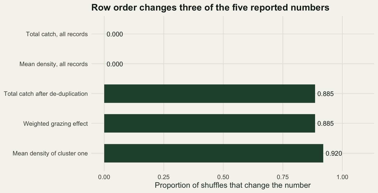
Three of the five reported numbers move. The total catch over all records and the mean density over all records are identical in every shuffle, which is worth saying plainly because the usual worry about summing floating point numbers in different orders is misplaced at this size: base R accumulates sums in extended precision, and the total over these records comes back bit for bit identical however the rows are arranged. The order dependence is not in the arithmetic.
It is in the de-duplication. Removing repeated records keeps the first occurrence of each site and round, and after a shuffle the first occurrence is a different record. The total catch that survives de-duplication ranges from 1429 to 1462 beetles across the shuffles, and the weighted grazing effect takes 8 distinct values spanning 11.5310 percentage points, from 61.5786 to 73.1096. The estimate that goes in the abstract therefore depends on the order in which two field books were pasted together, and the line responsible is a single call that most readers would pass over without a second glance.
The fifth number fails for a different reason, and it is worth isolating, because in the sweep above the clustering is fed by site densities that the de-duplication has already moved. The next block holds the site table fixed and shuffles only its rows.
tab_site <- data.frame(site = names(e_fixed$site_dens),
                       dens = as.numeric(e_fixed$site_dens),
                       rich = as.numeric(e_fixed$site_rich))
cluster_of <- function(tt) {
  g <- cutree(hclust(dist(scale(cbind(tt$dens, tt$rich)))), k = 2)
  names(g) <- tt$site
  g
}
g_file <- cluster_of(tab_site)
mates <- function(g) sort(names(g)[g == g[["S01"]]])

set.seed(20260813)
perm_lab <- t(replicate(200, {
  tt <- tab_site[sample(nrow(tab_site)), ]
  g <- cluster_of(tt)
  c(label = g[["S01"]],
    same_partition = as.numeric(identical(mates(g), mates(g_file))),
    cluster_one = mean(tab_site$dens[match(names(g)[g == 1], tab_site$site)]))
}))

print(table(g_file))
g_file
1 2
5 7 c(permutations = nrow(perm_lab),
identical_partitions = sum(perm_lab[, "same_partition"]),
label_of_S01_group_one = sum(perm_lab[, "label"] == 1),
label_of_S01_group_two = sum(perm_lab[, "label"] == 2)) permutations identical_partitions label_of_S01_group_one
200 200 89
label_of_S01_group_two
111 round(sort(unique(perm_lab[, "cluster_one"])), 4)[1] 255.1463 383.6873The partition is identical in all 200 permutations: the same five sites group together every time, so the ecology the clustering finds is stable. The integer the sites are labelled with is not, because cutree numbers the groups by the order in which their members appear in the input. Site S01 is in group one in 89 of the permutations and group two in the other 111. Any line that reports a property of group one is therefore reporting a property of whichever group happened to contain the first row, and the mean density of cluster one alternates between 255.1463 and 383.6873 beetles per hundred trap nights depending on nothing but the sort order of the table.
The general form of this failure is that the operation looks symmetric and is not. De-duplication keeps the first. Cluster labels follow the first. Ties in which.max, sort and order go to the first. Any resampling indexes positions rather than rows. None of these is a bug in R, and none of them announces itself, so the check is to shuffle and compare rather than to read the code looking for suspects.
Check 4: does the reported number match the computed number?
The last check is the one this blog runs on itself. Every number in the prose of a post is supposed to appear in the output of a chunk, rounded and not truncated, so that no sentence can drift away from the code that produced it. That rule is only worth having if something enforces it, and the enforcement is short enough to write out.
The checker splits a rendered document into code and prose at the fences, collects every number the code blocks printed, and asks of every number in the prose whether some printed value agrees with it when rounded to the number of decimals the prose used. Integers of ten or less are skipped, because they are almost always structural: the number of checks, the number of panels, the number of treatments.
num_of <- function(x) regmatches(x, gregexpr("-?[0-9]+(\\.[0-9]+)?", x))
word_val <- c(one = 1, two = 2, three = 3, four = 4, five = 5, six = 6, seven = 7,
              eight = 8, nine = 9, ten = 10, eleven = 11, twelve = 12, fifteen = 15,
              sixteen = 16, eighteen = 18, twenty = 20)

gate <- function(lines, use_abs = FALSE, use_scale = FALSE, use_words = FALSE) {
  fence <- grepl("^```", lines)
  in_code <- fence | (cumsum(fence) %% 2 == 1)
  printed <- as.numeric(unlist(num_of(lines[in_code])))
  prose <- lines[!in_code]
  tok <- unlist(num_of(prose))
  tok <- tok[grepl("\\.", tok) | abs(as.numeric(tok)) > 10]
  cand <- if (use_scale) c(printed, 100 * printed, printed / 100) else printed
  if (use_abs) cand <- abs(cand)
  miss <- character(0)
  for (k in tok) {
    x <- as.numeric(k); if (use_abs) x <- abs(x)
    d <- if (grepl("\\.", k)) nchar(sub("^[^.]*\\.", "", k)) else 0
    if (!any(abs(cand - x) <= 0.5 * 10^(-d) + 1e-9)) miss <- c(miss, k)
  }
  if (use_words) for (w in names(word_val))
    if (any(grepl(paste0("\\b", w, "\\b"), prose)) &&
        !any(abs(cand - word_val[[w]]) <= 0.5 + 1e-9)) miss <- c(miss, w)
  miss
}
c(lines_of_code = 20)
lines_of_code
20 A checker is only as good as the measurement of its error rate, so the next block builds a corpus with a known answer: six documents, each a run of prose sentences around one printed block, in which every prose number is planted deliberately and labelled. Forty of them simply agree with what was printed. Nine are legitimate sign flips, where the code printed a negative difference and the sentence says the same thing in words, so the digits carry no sign. Seven are legitimate scale changes, where the code printed a proportion and the sentence gives a percentage. Six are truncated instead of rounded, six are stale numbers from an earlier run, one has the sign genuinely wrong, four are stale numbers written out as words, and six are ordinary English sentences that happen to contain a number word.
set.seed(20260813)
pool <- round(runif(400, 12, 480), 4)
pool <- pool[!duplicated(round(pool, 1))]
is_tr <- (pool * 10) %% 1 >= 0.5
tr <- pool[is_tr][1:6]
pl <- pool[!is_tr][1:63]

claim <- function(x, kind) {
  out <- switch(kind,
    match   = data.frame(printed = sprintf("%.4f", x),  token = sprintf("%.4f", x)),
    sign    = data.frame(printed = sprintf("%.4f", -x), token = sprintf("%.4f", x)),
    signerr = data.frame(printed = sprintf("%.4f", -x), token = sprintf("%.4f", x)),
    percent = data.frame(printed = sprintf("%.4f", x / 1000), token = sprintf("%.2f", x / 10)),
    trunc   = data.frame(printed = sprintf("%.4f", x),
                         token = sprintf("%.1f", floor(x * 10) / 10)),
    stale   = data.frame(printed = sprintf("%.4f", x), token = sprintf("%.4f", x * 1.07)))
  out$kind <- kind
  out$err <- kind %in% c("signerr", "trunc", "stale")
  out
}
claims <- rbind(claim(pl[1:40], "match"), claim(pl[41:49], "sign"),
                claim(pl[50:56], "percent"), claim(tr, "trunc"),
                claim(pl[57:62], "stale"), claim(pl[63], "signerr"))
words <- data.frame(printed = c("12", "18", "9", "16"),
                    token = c("ten", "fifteen", "eight", "twenty"),
                    kind = "word", err = TRUE)
english <- data.frame(printed = "", token = c("one", "two", "three", "four", "five", "six"),
                      kind = "english", err = FALSE)

tmpl <- c("The weighted mean catch per unit effort came out at TOK.",
          "The grazed sites sit at TOK on the same scale.",
          "That leaves a treatment contrast of TOK.",
          "The upper limit of the interval sits at TOK.",
          "Across the sites the spread of the estimate was TOK.",
          "The permutation statistic came out at TOK.",
          "The site level standard deviation was TOK.",
          "Dropping the weakest site moves the estimate to TOK.")
eng_line <- c("There is more than one way to read that table.",
              "The two panels share a vertical scale.",
              "All three mechanisms depend on the order of the rows.",
              "The four checks cost minutes to run.",
              "Only five of the sites were resurveyed.",
              "The six sections that follow are independent.")

n_doc <- 6
claims$doc <- rep(1:n_doc, length.out = nrow(claims))
words$doc <- 1:4
english$doc <- 1:n_doc

build <- function(i) {
  cl <- claims[claims$doc == i, ]; wd <- words[words$doc == i, ]
  pr <- mapply(function(t, k) sub("TOK", k, t),
               rep(tmpl, length.out = nrow(cl)), cl$token, USE.NAMES = FALSE)
  if (nrow(wd)) pr <- c(pr, paste0("The design has ", wd$token, " paired replicates."))
  pr <- c(pr, eng_line[english$doc == i])
  c(pr[1:2], "```", paste(c(cl$printed, wd$printed), collapse = " "), "```", pr[-(1:2)])
}
corpus <- lapply(1:n_doc, build)
truth <- rbind(claims[, c("token", "kind", "err")], words[, c("token", "kind", "err")],
               english[, c("token", "kind", "err")])

c(documents = n_doc, claims = nrow(truth), distinct_tokens = length(unique(truth$token)),
  planted_errors = sum(truth$err))
documents claims distinct_tokens planted_errors
6 79 79 17 print(table(truth$kind))
english   match percent    sign signerr   stale   trunc    word
6 40 7 9 1 6 6 4 cat(corpus[[2]][1:6], sep = "\n")The weighted mean catch per unit effort came out at 253.7069.
The grazed sites sit at 296.6055 on the same scale.
```
253.7069 296.6055 87.1368 221.6128 135.8281 302.0102 448.4499 -255.4320 0.4205 0.1011 304.4549 453.5001 18
```
That leaves a treatment contrast of 87.1368.Now the measurement. Four versions of the checker are run over the corpus: the plain one, the one that compares on absolute value, the one that also tries the value multiplied and divided by a hundred, and the one that additionally reads number words.
score <- function(...) {
  fl <- unique(unlist(lapply(corpus, gate, ...)))
  hit <- truth$token %in% fl
  c(flagged = length(fl), caught = sum(hit & truth$err),
    false_alarms = sum(hit & !truth$err), missed = sum(!hit & truth$err))
}
result <- rbind(plain = score(),
                absolute_value = score(use_abs = TRUE),
                plus_scale = score(use_abs = TRUE, use_scale = TRUE),
                plus_words = score(use_abs = TRUE, use_scale = TRUE, use_words = TRUE))
print(result)
flagged caught false_alarms missed
plain 29 13 16 4
absolute_value 19 12 7 5
plus_scale 12 12 0 5
plus_words 18 16 2 1flag_plain <- unique(unlist(lapply(corpus, gate)))
flag_full <- unique(unlist(lapply(corpus, gate, use_abs = TRUE, use_scale = TRUE)))
flag_word <- unique(unlist(lapply(corpus, gate, use_abs = TRUE, use_scale = TRUE,
use_words = TRUE)))
by_kind <- t(sapply(unique(truth$kind), function(k) {
s <- truth$kind == k
c(n = sum(s), plain = sum(truth$token[s] %in% flag_plain),
plus_scale = sum(truth$token[s] %in% flag_full),
plus_words = sum(truth$token[s] %in% flag_word))
}))
print(by_kind) n plain plus_scale plus_words
match 40 0 0 0
sign 9 9 0 0
percent 7 7 0 0
trunc 6 6 6 6
stale 6 6 6 6
signerr 1 1 0 0
word 4 0 0 4
english 6 0 0 2gl <- data.frame(
version = factor(rep(c("Plain", "Absolute value", "Plus scale", "Plus number words"),
times = 3),
levels = rev(c("Plain", "Absolute value", "Plus scale",
"Plus number words"))),
outcome = factor(rep(c("Errors caught", "False alarms", "Errors missed"), each = 4),
levels = c("Errors caught", "False alarms", "Errors missed")),
count = c(result[, "caught"], result[, "false_alarms"], result[, "missed"]))
ggplot(gl, aes(count, version, fill = outcome)) +
geom_col(position = position_dodge(width = 0.72), width = 0.66) +
geom_text(aes(label = count), position = position_dodge(width = 0.72),
hjust = -0.4, colour = te_pal$ink, size = 3.2) +
scale_x_continuous(limits = c(0, 18.5), breaks = seq(0, 18, by = 3)) +
scale_fill_manual(values = c(te_pal$forest, te_pal$clay, te_pal$gold), name = NULL) +
labs(x = "Prose numbers", y = NULL,
title = "Two fixes clear the false alarms and leave a blind spot") +
theme_te() +
theme(legend.position = "top")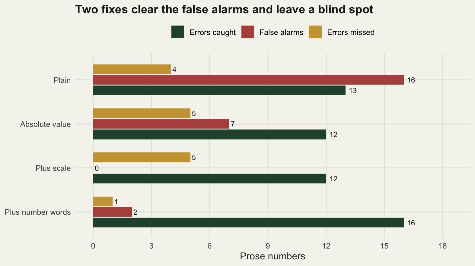
The plain version flags 29 prose numbers. Of those, 13 are real errors and 16 are false alarms, which is a ratio that guarantees the checker gets switched off within a week. Every one of the false alarms comes from a sentence that is correct English: 9 of them state the size of a negative quantity without repeating the minus sign, which is what a sentence saying that one treatment is lower than another does, and 7 give a percentage where the code printed a proportion.
Comparing on absolute value removes the first 9. Adding the scaled candidates removes the other 7, and the checker then flags 12 numbers, all of them real: the 6 truncations and the 6 stale values. The price of the first fix is exact and it is worth naming. The corpus contains one sentence whose sign is genuinely wrong, a decrease written up as an increase. The plain version catches it, because the digits are unsigned in the prose and negative in the output; the absolute value version cannot, because it has thrown away the only evidence there was. A checker that reads digits and not English cannot tell a legitimate sign flip from an illegitimate one, so it must choose which error to make, and 9 false alarms against 1 catch is not a close decision.
The second finding is the one that costs a figure caption. Of the 17 planted errors, 4 are written out as words: a caption saying the design has ten paired replicates when the code now prints 12, and three like it. No version that reads digits can see them, and this is exactly how a stale caption survives a rewrite. Teaching the checker the number words up to twenty catches all 4 of them, and it raises 2 false alarms in 6 ordinary English sentences: the last two versions differ by nothing else. Worse, the 4 sentences that pass do so by luck rather than by correctness, because one of the candidate values, or that value scaled by a hundred, happened to land within half a unit of the word. A rule that passes for the wrong reason will fail for the wrong reason on the next post.
The practical answer is not a better checker. It is to write every number that carries a result as digits, keep the words for quantities that are not results, and accept that the checker enforces the digits rule rather than the truth.
The honest limit
Every check in this post compares the script with itself. Check 1 asks whether two runs of the same code agree. Check 2 asks whether two runs with the same seed agree. Check 3 asks whether two orders of the same rows agree. Check 4 asks whether the prose agrees with the output. Not one of them asks whether the analysis is the right analysis, and a script can pass all four while answering the wrong question perfectly.
The transcription slips make the point. Once the correction is written into the script rather than typed at the console, Check 1 passes on both versions of it: the one that divides by two trap nights and the one that divides by eight. The check certifies that 118.6719 per cent is what the code computes, which is true, and says nothing about the fact that three rows of the data are wrong. That belongs to a different family of checks, the ones that compare the data with the field sheets and the model with the biology, and no amount of session hygiene substitutes for it.
There is also a cost side that this post has not priced. Running from a clean session takes as long as the analysis takes, which for a large model is not a habit you can keep on every save. The practical compromise is the one the reproducible workflow post argues for: cheap checks continuously, the expensive full rerun at the points where the work leaves your hands, and a recorded seed so that the expensive rerun is a rerun rather than a new experiment.
Where to go next
The four checks here take minutes and want to be routine rather than heroic. Put the clean session run in front of anything you send to a co-author, seed each stochastic block rather than the script, shuffle the rows once before you believe a number, and write results as digits so that a twenty line checker can see them.
For the surrounding habits, a reproducible statistical workflow in R sets out the project layout and the rendering discipline these checks assume, and testing your analysis code turns the informal checks here into assertions that fail loudly when a function stops doing what it did. Debugging and defensive R code is the place to go when a check comes back positive and you have to find out why.
References
Peng RD 2011 Science 334(6060):1226-1227 (10.1126/science.1213847)
Sandve GK, Nekrutenko A, Taylor J, Hovig E 2013 PLoS Computational Biology 9(10):e1003285 (10.1371/journal.pcbi.1003285)
Wilson G, Bryan J, Cranston K, Kitzes J, Nederbragt L, Teal TK 2017 PLoS Computational Biology 13(6):e1005510 (10.1371/journal.pcbi.1005510)
Matsumoto M, Nishimura T 1998 ACM Transactions on Modeling and Computer Simulation 8(1):3-30 (10.1145/272991.272995)
Goldberg D 1991 ACM Computing Surveys 23(1):5-48 (10.1145/103162.103163)
Powers SM, Hampton SE 2019 Ecological Applications 29(1):e01822 (10.1002/eap.1822)