library(boot)
library(ggplot2)

paper <- "#f5f4ee"; ink <- "#16241d"; forest <- "#275139"
gold  <- "#cda23f"; off_red <- "#b5534e"; faint <- "#5d6b61"; line <- "#dad9ca"

theme_te <- theme_minimal(base_size = 12) +
  theme(panel.grid.minor = element_blank(),
        panel.grid.major = element_line(colour = line, linewidth = 0.3),
        plot.background = element_rect(fill = paper, colour = NA),
        panel.background = element_rect(fill = paper, colour = NA),
        axis.title = element_text(colour = ink),
        axis.text = element_text(colour = faint),
plot.title = element_text(colour = ink, face = "bold"))A reproducible statistical workflow in R
reproducibility
workflow
ecology tutorial
R
Making an ecological analysis reproducible in R: seeding random steps, recording package versions, using relative paths, and rendering from a clean session.
An analysis is reproducible when someone else, or you in six months, can run the same code on the same data and get the same numbers. That sounds automatic, but it rarely is. Random steps give different answers each run, a package update silently changes a default, an absolute file path breaks on another machine, and a result that depended on objects left over in your session vanishes when the session is clean. None of these are exotic. They are the ordinary ways an ecological analysis stops reproducing, and each has a short, boring fix. This post walks through the four that matter most.
Seed every random step
Permutation tests, bootstraps, simulations, and random subsampling all draw on R’s random number generator, and without a fixed starting point they give a different answer every run. set.seed() fixes that starting point. Call it directly before the random step, not once at the top of a long script, so it is obvious which result each seed controls and so that reordering code does not quietly change the numbers.
draw <- function(seed) { set.seed(seed); rnorm(5) }

identical(draw(42), draw(42))     # same seed, same numbers
[1] TRUEidentical(draw(42), draw(99)) # different seed, different numbers[1] FALSEThe same discipline makes a whole bootstrap reproducible. Fix one seed for the data and another immediately before the resampling, and the confidence interval is identical on every run.
boot_ci <- function(boot_seed) {
  set.seed(123)                                   # the data, fixed
  x <- rgamma(40, 4, 0.2)
  set.seed(boot_seed)                             # the resampling, fixed
  b <- boot(x, function(d, i) mean(d[i]), R = 2000)
  as.numeric(boot.ci(b, type = "perc")$percent[4:5])
}
run_A <- boot_ci(7)
run_B <- boot_ci(7)
list(run_A = round(run_A, 3), identical = identical(run_A, run_B))
$run_A
[1] 15.100 19.832
$identical
[1] TRUEBoth runs return the interval 15.1 to 19.83, and identical() confirms they match to the last digit. The figure makes the contrast visible: when two runs share a seed every replicate lands exactly on the diagonal, and when the seeds differ the replicates scatter into an uninformative cloud.
set.seed(2024); r1 <- replicate(150, mean(sample(rnorm(30), replace = TRUE)))
set.seed(2024); r2 <- replicate(150, mean(sample(rnorm(30), replace = TRUE)))
set.seed(7777); r3 <- replicate(150, mean(sample(rnorm(30), replace = TRUE)))

fig <- rbind(
  data.frame(run1 = r1, run2 = r2, seed = "same seed"),
  data.frame(run1 = r1, run2 = r3, seed = "different seed")
)

ggplot(fig, aes(run1, run2, colour = seed)) +
  geom_abline(slope = 1, intercept = 0, colour = ink, linewidth = 0.4) +
  geom_point(size = 1.6, alpha = 0.8) +
  scale_colour_manual(values = c("same seed" = gold, "different seed" = off_red)) +
  labs(x = "replicate mean, run 1", y = "replicate mean, run 2",
       colour = NULL, title = "Same seed reproduces; different seed does not") +
  theme_te + theme(legend.position = "top")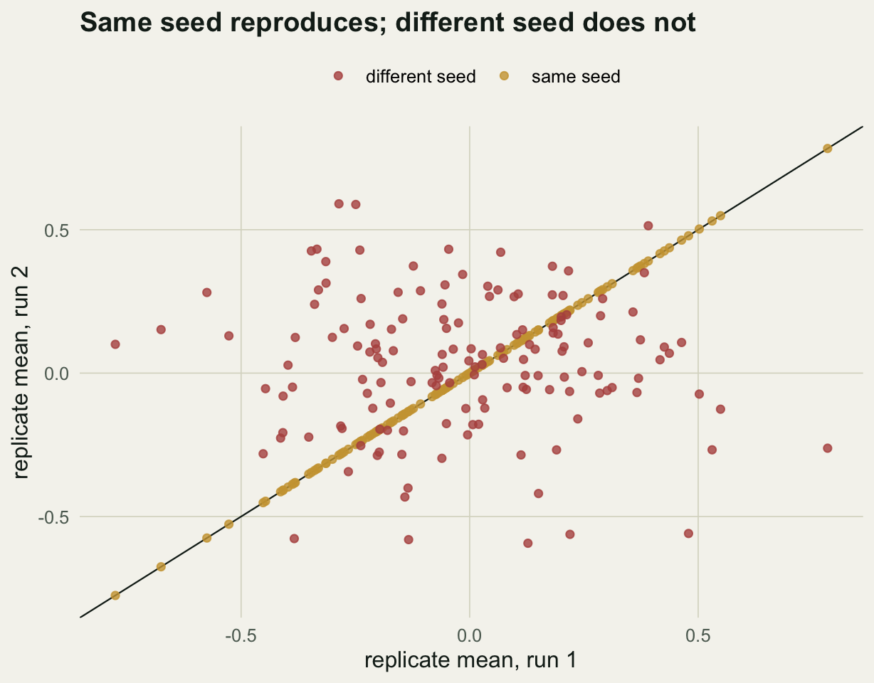
Record the session and the package versions
Code reproduces against a moving target: R itself and every package keep changing, and a new default can shift your results without any change to your script. Record the versions you actually ran, so a future reader knows what to match.
R.version.string[1] "R version 4.5.3 (2026-03-11)"vapply(c("boot", "ggplot2", "vegan"),
function(p) as.character(packageVersion(p)), character(1)) boot ggplot2 vegan
"1.3.32" "4.0.3" "2.7.5" Pasting sessionInfo() at the end of a report is the minimum. For a project you intend to revisit or share, the renv package goes further: it records the exact version of every package in a lockfile and can reinstall that precise set later, so the analysis runs against the libraries it was written for rather than whatever happens to be installed.
Use paths that survive a move
A path like setwd("/Users/me/Desktop/fieldwork") works on exactly one machine and breaks everywhere else. Keep all paths relative to the project root instead, so the same code runs wherever the project folder lands. The here package resolves paths from the project root automatically, and a tidy layout keeps the pieces separate, for example raw data under data/, code under R/, and generated output under output/. Reading with here::here("data", "sites.csv") rather than an absolute path is the single change that lets a collaborator clone the project and run it without editing a line.
Render from a clean session
The most common hidden dependency is an object that exists in your session but is not created by your script: a data frame you loaded by hand, a variable from an experiment you forgot to delete. The analysis works for you and fails for everyone else. The test is simple: restart R to clear everything, then run the whole analysis from the top. If it completes and the numbers match, the script is self-contained. Quarto and R Markdown enforce this by rendering in a fresh session every time, which is most of why they are worth using. Quarto’s freeze option records computed results so a document rebuilds without rerunning every analysis, while still guaranteeing the output came from the code in front of you rather than from forgotten session state.
What to carry forward
Reproducibility is not a separate virtuous task bolted on at the end; it is a handful of habits that cost almost nothing during the work. Seed every random step, and seed it next to the step. Record the R and package versions you ran, and pin them with renv for anything you will return to. Keep paths relative to the project root. Render from a clean session, or let Quarto do it for you, so that hidden state cannot prop up a result. Do these and the analysis will still produce its numbers long after you have forgotten how it works, which is the whole point.
References
Sandve GK, Nekrutenko A, Taylor J, Hovig E 2013 PLoS Computational Biology 9(10):e1003285 (10.1371/journal.pcbi.1003285)
Wilson G, Bryan J, Cranston K, Kitzes J, Nederbragt L, Teal TK 2017 PLoS Computational Biology 13(6):e1005510 (10.1371/journal.pcbi.1005510)