---
title: "Exporting publication-quality ggplot figures in R"
description: "Save ggplot2 figures that meet journal rules: setting physical size and resolution, choosing PNG, TIFF, PDF or SVG, and embedding fonts so your text survives."
date: "2026-05-04 12:00"
categories: [R, data visualisation, ggplot2, workflow, ecology tutorial]
image: thumbnail.png
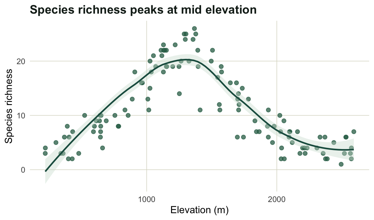
image-alt: "An ecology scatter plot of species richness against elevation, used as the example figure for export."
---
You have a figure you are happy with. Then the submission portal asks for 300 dpi, a width of exactly 85 mm, fonts embedded, and a vector file if possible. The good news is that `ggsave` does all of this from a few arguments, and you never have to screenshot a plot again. This post walks through the settings that matter, using one ecology figure as the running example.
```{r}
#| label: figure
#| message: false
#| warning: false
#| fig-width: 6.3
#| fig-height: 3.7
#| fig-cap: "The example figure: simulated species richness along an elevation gradient, with a loess smoother. It sits on white here, not on the page colour the other figures on this site use, because white is what the journal will print."
#| fig-alt: "A scatter of simulated species richness against elevation with a loess smoother through the points, drawn on a plain white background."
library(ggplot2)

set.seed(7)
elev <- runif(120, 200, 2600)
rich <- rpois(120, exp(1.4 + 1.7 * exp(-((elev - 1300) / 600)^2)))
df <- data.frame(elev, rich)

p <- ggplot(df, aes(elev, rich)) +
  geom_point(color = "#2f6d54", alpha = 0.75, size = 2) +
  geom_smooth(method = "loess", formula = y ~ x, se = TRUE,
              color = "#1d5b4e", fill = "#cfe0d4", linewidth = 0.9) +
  labs(x = "Elevation (m)", y = "Species richness",
       title = "Species richness peaks at mid elevation") +
  theme_minimal(base_size = 12) +
  theme(panel.grid.minor = element_blank(),
        panel.grid.major = element_line(color = "#dad9ca", linewidth = 0.3),
        plot.title = element_text(face = "bold", color = "#16241d"))
p
```
One deliberate difference from the rest of this site: the figure above is drawn on white. Every other figure here sits on the page colour so that it reads as part of the page, but a submitted figure is not part of a page you control, and a tinted canvas will either be printed as a grey rectangle or asked about in production. Leave the background white in anything you are going to send, and let the journal supply the surround.
## Size and resolution
The two arguments that decide everything are the physical size (`width`, `height`, with `units`) and, for raster output, the resolution (`dpi`). Set the size to the space the figure will occupy in print, not to whatever looks right on screen. Most journals use a single-column width near 85 mm and a double-column width near 170 mm. For resolution, 300 dpi is the usual minimum for plots with shading or colour, and 600 dpi or more is asked for line art where thin strokes must stay crisp.
The pixel dimensions of a raster file are just the physical size times the resolution. A figure 85 mm wide at 300 dpi is `85 / 25.4 * 300`, just under 1004 pixels across, which the device writes out as 1003. We can write the file and read the dimensions back to confirm it.
```{r}
#| label: resolution
out <- tempdir()
ggsave(file.path(out, "fig_300.png"), p, width = 85, height = 85, units = "mm", dpi = 300)
ggsave(file.path(out, "fig_600.png"), p, width = 85, height = 85, units = "mm", dpi = 600)

png_dim <- function(f) {                       # read width and height from the PNG header
  x <- readBin(f, "integer", n = 6, size = 4, endian = "big")
  c(width = x[5], height = x[6])
}
rbind(`300 dpi` = png_dim(file.path(out, "fig_300.png")),
      `600 dpi` = png_dim(file.path(out, "fig_600.png")))
```
The 300 dpi file is about 1003 pixels square and the 600 dpi file is twice that on each side. Doubling the resolution quadruples the pixel count and the file size, so do not ask for 600 dpi unless the figure needs it.
## Prefer vector when you can
A raster file (PNG, TIFF) is a fixed grid of pixels: zoom in far enough and you see the squares. A vector file (PDF, SVG) stores the lines and text as instructions, so it stays sharp at any size and the text remains real text. For scatter plots, line plots, and anything text-heavy, vector is the better choice when the journal accepts it, and the files are usually smaller too.
```{r}
#| label: vector
# cairo_pdf embeds and subsets the fonts; fall back if this R was built without cairo
pdf_device <- if (isTRUE(capabilities("cairo"))) cairo_pdf else pdf
ggsave(file.path(out, "fig.pdf"), p, width = 85, height = 85, units = "mm",
       device = pdf_device)
ggsave(file.path(out, "fig.svg"), p, width = 85, height = 85, units = "mm")
ggsave(file.path(out, "fig.tiff"), p, width = 85, height = 85, units = "mm",
       dpi = 300, compression = "lzw")

files <- c("fig_300.png", "fig.tiff", "fig.pdf", "fig.svg")
data.frame(file = files,
           kb = round(file.size(file.path(out, files)) / 1024, 1))
```
The PDF and SVG come out a fraction of the size of the raster files and will print sharply at any scale. TIFF is the format some journals still insist on; use LZW compression to keep it from ballooning.
## Embed your fonts
Here is the trap that bites people after acceptance. The base PDF device does not embed fonts by default, so a reader (or a typesetter) without your exact font sees a substitute, and labels can shift or break. The `cairo_pdf` device embeds and subsets the fonts into the file, which is why we used it above. You can confirm it from a terminal with `pdffonts fig.pdf`: the font shows up with `emb` set to yes. For SVG, the `svglite` device writes clean, standards-compliant files, and most submission systems handle them well.
If a publisher cannot accept embedded fonts at all, the fallback is to convert the text to outlines (paths) so it no longer depends on a font being present. Reaching for `cairo_pdf` first avoids the problem in nearly every case.
## A small recipe
For day-to-day work it helps to wrap the common cases in one function, so every figure in a manuscript comes out at the same size and quality.
```{r}
#| label: recipe
save_fig <- function(plot, name, width = 85, height = 85, dpi = 300) {
  ggsave(paste0(name, ".pdf"), plot, width = width, height = height,
         units = "mm", device = cairo_pdf)                       # vector master
  ggsave(paste0(name, ".png"), plot, width = width, height = height,
         units = "mm", dpi = dpi)                                 # raster preview
  invisible(name)
}
# save_fig(p, file.path(tempdir(), "richness_elevation"), width = 170)
```
Keep a vector master and a raster preview of every figure, set the width to the column it will sit in, and let the journal tell you which file to upload. With the size and device fixed up front, a revision is one call, not an afternoon in an image editor.
## References
Wickham H 2016 ggplot2: Elegant Graphics for Data Analysis, 2nd edition, Springer, Cham (10.1007/978-3-319-24277-4)
Wickham H, Henry L, Pedersen TL, Luciani TJ, Decorde M, Lise V 2023 svglite: An SVG Graphics Device, R package version 2.1.3 (https://CRAN.R-project.org/package=svglite)
## Related tutorials
- [A reproducible statistical workflow](../reproducible-statistical-workflow/)
- [Bootstrap confidence intervals](../bootstrap-confidence-intervals/)
- [Standard errors and confidence intervals](../standard-errors-confidence-intervals/)
- [Checking a figure](../checking-a-figure/)