A first R session for ecologists: RStudio projects instead of setwd, installing packages once, and why a clean-session script is the only reproducible analysis.
Corrected 15 October 2026: the post said RStudio opens with four panes; on a first start it shows three, and the script editor opens above the console once a script is opened or created, as the text now says.
Corrected 30 September 2026: the post said a script that runs after Session then Restart R draws only on the script; it now adds that this holds only when RStudio is set not to restore or save the workspace, since a saved .RData file can bring stale objects back.
Most ecology tutorials start with the data already loaded, as if the counts arrive in your R session by magic. They do not. Before any diversity index or ordination, you have to open R, point it at a folder of field data, load the packages you need, and run your code in a way that you (or a reviewer, or you in six months) can reproduce. That last part is where most beginner workflows quietly break, and it has nothing to do with statistics.
This post sets up a working session the way a careful analysis needs it: an RStudio project instead of a hard-coded path, packages installed once and loaded every time, and a script rather than a stream of console commands. The payoff is concrete, so we finish by watching a leftover value in the workspace silently change a diversity estimate.
The console is for trying things; the script is the analysis
When you first open RStudio you get three panes; a fourth, the script editor, opens above the console once you open or create a script (File then New File then R Script). The one that matters first is the console (on the left), where you type a line and R answers immediately. It is ideal for trying something out. It is a poor place to keep an analysis, because the console has a memory you cannot see and a colleague cannot reproduce.
The script editor (top left) is where the analysis lives. You write your commands in a .R file (or a Quarto document), save it, and run it top to bottom. The difference is not cosmetic. A script is a record: anyone with the script and the data can get your numbers. A console session is a conversation that vanishes when you close R.
A useful habit from day one: type exploratory lines in the console, but the moment a line becomes part of the analysis, move it into the script. If it is not in the script, it did not happen.
Projects, not setwd()
The single most common reason a colleague cannot run your script is a line like this:
setwd("C:/Users/alice/Documents/fieldwork/2025/")
That path exists on exactly one computer. On anyone else’s machine the script fails on line 1, and even on your own machine it breaks the moment you move the folder or rename it.
The fix is an RStudio project. In RStudio choose File then New Project, and make a project folder for your study (say, meadow-survey/). RStudio drops a small .Rproj file in it and, importantly, sets the working directory to that folder every time you open the project. Now your data lives at a relative path:
counts <-read.csv("data/plot-counts.csv")
There is no drive letter and no username. The same line works on your laptop, your supervisor’s desktop, and the machine that renders the analysis. Keep the raw data in a data/ subfolder, your scripts in the project root, and never write setwd() again. (For the broader habits that make an analysis rerun cleanly, see the reproducible-workflow tutorial linked at the end.)
Install once, load every session
Two verbs trip up every beginner because they look interchangeable and are not.
install.packages("vegan") downloads a package from CRAN and copies it onto your computer. You do this once (and again when you want a newer version). It does not belong in your analysis script, because rerunning it re-downloads the package every time.
library(vegan) makes an already-installed package available in the current session. R starts each session with only the base packages loaded, so you call library() at the top of every script, for every package you use. Group the library() calls at the top; leave install.packages() out of the script, or comment it out.
# install.packages(c("vegan", "dplyr")) # run once, by hand, then comment outlibrary(vegan)library(dplyr)
If a script errors with there is no package called 'vegan', you skipped the install. If it errors with could not find function "diversity", you skipped the library().
Why the clean session matters: a leftover value
Here is the measurable point, and it is the reason the console-versus-script distinction is more than tidiness. We compute Shannon diversity for one plot. The data is four species and their counts:
The correct total is 26 individuals and the Shannon value is 1.162. Now picture the ordinary way beginners work. Earlier in the console, for a different plot, you had typed N <- 40. You then write the script above but forget the line N <- sum(counts). Because N is still sitting in the workspace as 40, the script runs without complaint:
# the workspace still holds N <- 40 from an earlier, different plotN_stale <-40p_stale <- counts / N_stale # divides by the wrong totalH_stale <--sum(p_stale *log(p_stale))round(H_stale, 3) # a Shannon value, but the wrong one
[1] 1.035
The script produced 1.035 instead of the correct 1.162, a 10.9 per cent error, with no warning of any kind. The only hint that something is off is that the relative abundances now sum to 0.65 rather than 1, and nothing forces you to notice.
Run the same script in a fresh session, where N was never defined, and R stops you:
clean <-new.env(parent =baseenv()) # an empty workspace, as a fresh session would haveclean$counts <- countsresult <-tryCatch(eval(quote(counts / N), envir = clean), # N does not exist hereerror =function(e) conditionMessage(e))result
[1] "object 'N' not found"
The clean session turns a silent wrong answer into a loud, fixable error. This is the whole argument for the workflow above: “it ran on my machine” is not the same as “it is correct”, because your machine remembers things your script never wrote down. In RStudio the check is one menu item, Session then Restart R, followed by running the script from the top (Run then Run All). If it fails, you found a hidden dependency. If it runs, your numbers came from the script and nothing else, provided the restarted session really is empty: in Tools then Global Options then General, untick restoring .RData into the workspace at startup and set saving the workspace on exit to Never, or a saved workspace can bring the stale N back.
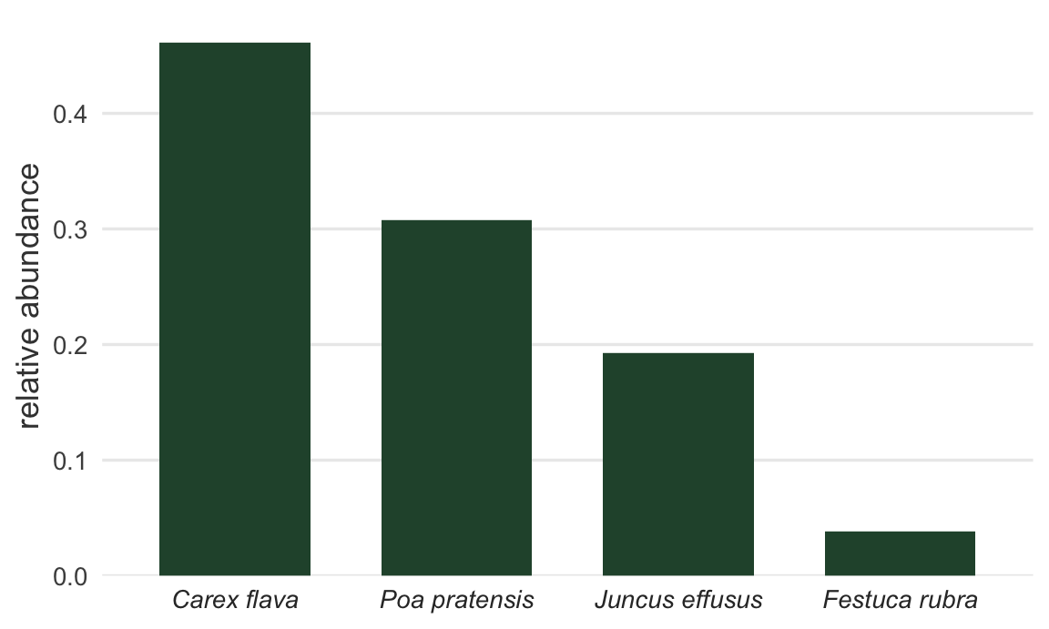
Figure 1: Relative abundance of the four species in the plot. This community profile is what a Shannon value summarises into one number, and dividing it by the wrong total (a stale workspace value) distorts every bar.
Where to go next
You now have a project, a script, and a session you can restart with confidence. The next step is getting real field data into that session, where the first surprise is that a blank cell is not a zero. The reading-field-data tutorial picks up exactly there.
References
Wickham H, Grolemund G 2017. R for Data Science. O’Reilly. ISBN 978-1-491-91039-9.
R version 4.5.3 (2026-03-11), aarch64-apple-darwin20
Packages: dplyr 1.2.1, ggplot2 4.0.3
Newsletter
Get updates by email
An occasional email when tutorials are added or substantially corrected. No spam; unsubscribe anytime.
By subscribing you agree to receive these emails and confirm your address once. See the privacy policy.
ESC
Type to search the tutorials
Source Code
---title: "Setting up R and RStudio for ecology"description: "A first R session for ecologists: RStudio projects instead of setwd, installing packages once, and why a clean-session script is the only reproducible analysis."date: "2026-06-18 14:00"date-modified: "2026-10-15"categories: [R, RStudio, reproducibility, ecology tutorial]image: thumbnail.pngimage-alt: "Bar chart of the relative abundance of four plant species in one field plot."---*Corrected 15 October 2026: the post said RStudio opens with four panes; on a first start it shows three, and the script editor opens above the console once a script is opened or created, as the text now says.**Corrected 30 September 2026: the post said a script that runs after Session then Restart R draws only on the script; it now adds that this holds only when RStudio is set not to restore or save the workspace, since a saved .RData file can bring stale objects back.*Most ecology tutorials start with the data already loaded, as if the counts arrive in your R session by magic. They do not. Before any diversity index or ordination, you have to open R, point it at a folder of field data, load the packages you need, and run your code in a way that you (or a reviewer, or you in six months) can reproduce. That last part is where most beginner workflows quietly break, and it has nothing to do with statistics.This post sets up a working session the way a careful analysis needs it: an RStudio project instead of a hard-coded path, packages installed once and loaded every time, and a script rather than a stream of console commands. The payoff is concrete, so we finish by watching a leftover value in the workspace silently change a diversity estimate.## The console is for trying things; the script is the analysisWhen you first open RStudio you get three panes; a fourth, the script editor, opens above the console once you open or create a script (File then New File then R Script). The one that matters first is the **console** (on the left), where you type a line and R answers immediately. It is ideal for trying something out. It is a poor place to keep an analysis, because the console has a memory you cannot see and a colleague cannot reproduce.The **script editor** (top left) is where the analysis lives. You write your commands in a `.R` file (or a Quarto document), save it, and run it top to bottom. The difference is not cosmetic. A script is a record: anyone with the script and the data can get your numbers. A console session is a conversation that vanishes when you close R.A useful habit from day one: type exploratory lines in the console, but the moment a line becomes part of the analysis, move it into the script. If it is not in the script, it did not happen.## Projects, not setwd()The single most common reason a colleague cannot run your script is a line like this:```rsetwd("C:/Users/alice/Documents/fieldwork/2025/")```That path exists on exactly one computer. On anyone else's machine the script fails on line 1, and even on your own machine it breaks the moment you move the folder or rename it.The fix is an **RStudio project**. In RStudio choose File then New Project, and make a project folder for your study (say, `meadow-survey/`). RStudio drops a small `.Rproj` file in it and, importantly, sets the working directory to that folder every time you open the project. Now your data lives at a **relative** path:```rcounts <-read.csv("data/plot-counts.csv")```There is no drive letter and no username. The same line works on your laptop, your supervisor's desktop, and the machine that renders the analysis. Keep the raw data in a `data/` subfolder, your scripts in the project root, and never write `setwd()` again. (For the broader habits that make an analysis rerun cleanly, see the reproducible-workflow tutorial linked at the end.)## Install once, load every sessionTwo verbs trip up every beginner because they look interchangeable and are not.`install.packages("vegan")` downloads a package from CRAN and copies it onto your computer. You do this **once** (and again when you want a newer version). It does not belong in your analysis script, because rerunning it re-downloads the package every time.`library(vegan)` makes an already-installed package available in the **current** session. R starts each session with only the base packages loaded, so you call `library()` at the top of every script, for every package you use. Group the `library()` calls at the top; leave `install.packages()` out of the script, or comment it out.```r# install.packages(c("vegan", "dplyr")) # run once, by hand, then comment outlibrary(vegan)library(dplyr)```If a script errors with `there is no package called 'vegan'`, you skipped the install. If it errors with `could not find function "diversity"`, you skipped the `library()`.## Why the clean session matters: a leftover valueHere is the measurable point, and it is the reason the console-versus-script distinction is more than tidiness. We compute Shannon diversity for one plot. The data is four species and their counts:```{r}#| label: plot-countscounts <-c(`Carex flava`=12, `Juncus effusus`=5,`Poa pratensis`=8, `Festuca rubra`=1)N <-sum(counts) # this plot's total: 26 individualsp <- counts / N # relative abundancesH_correct <--sum(p *log(p)) # Shannon diversityround(H_correct, 3)```The correct total is `r sum(counts)` individuals and the Shannon value is `r sprintf("%.3f", -sum((counts/sum(counts))*log(counts/sum(counts))))`. Now picture the ordinary way beginners work. Earlier in the console, for a different plot, you had typed `N <- 40`. You then write the script above but forget the line `N <- sum(counts)`. Because `N` is still sitting in the workspace as 40, the script runs without complaint:```{r}#| label: stale-state# the workspace still holds N <- 40 from an earlier, different plotN_stale <-40p_stale <- counts / N_stale # divides by the wrong totalH_stale <--sum(p_stale *log(p_stale))round(H_stale, 3) # a Shannon value, but the wrong one``````{r}#| label: stale-numbers#| include: falseH_correct <--sum((counts /sum(counts)) *log(counts /sum(counts)))H_stale <--sum((counts /40) *log(counts /40))pct <- (H_stale - H_correct) / H_correct *100sum_stale <-sum(counts /40)```The script produced `r sprintf("%.3f", H_stale)` instead of the correct `r sprintf("%.3f", H_correct)`, a `r sprintf("%.1f", abs(pct))` per cent error, with no warning of any kind. The only hint that something is off is that the relative abundances now sum to `r sprintf("%.2f", sum_stale)` rather than 1, and nothing forces you to notice.Run the same script in a **fresh** session, where `N` was never defined, and R stops you:```{r}#| label: clean-sessionclean <-new.env(parent =baseenv()) # an empty workspace, as a fresh session would haveclean$counts <- countsresult <-tryCatch(eval(quote(counts / N), envir = clean), # N does not exist hereerror =function(e) conditionMessage(e))result```The clean session turns a silent wrong answer into a loud, fixable error. This is the whole argument for the workflow above: "it ran on my machine" is not the same as "it is correct", because your machine remembers things your script never wrote down. In RStudio the check is one menu item, Session then Restart R, followed by running the script from the top (Run then Run All). If it fails, you found a hidden dependency. If it runs, your numbers came from the script and nothing else, provided the restarted session really is empty: in Tools then Global Options then General, untick restoring .RData into the workspace at startup and set saving the workspace on exit to Never, or a saved workspace can bring the stale `N` back.```{r}#| label: fig-abundance#| echo: false#| fig-width: 6#| fig-height: 3.6#| fig-cap: "Relative abundance of the four species in the plot. This community profile is what a Shannon value summarises into one number, and dividing it by the wrong total (a stale workspace value) distorts every bar."#| fig-alt: "Bar chart of relative abundance for Carex flava, Poa pratensis, Juncus effusus and Festuca rubra, ordered tallest to shortest, with Carex flava tallest at about 0.46 and Festuca rubra shortest at about 0.04."library(ggplot2)te_green <-"#275139"df <-data.frame(species =names(counts),prop =as.numeric(counts) /sum(counts))df$species <-factor(df$species, levels = df$species[order(-df$prop)])ggplot(df, aes(x = species, y = prop)) +geom_col(fill = te_green, width =0.68) +scale_y_continuous(expand =expansion(mult =c(0, 0.05))) +labs(x =NULL, y ="relative abundance") +theme_minimal(base_size =13) +theme(plot.background =element_rect(fill ="#f5f4ee", colour =NA),panel.background =element_rect(fill ="#f5f4ee", colour =NA),panel.grid.minor =element_blank(),panel.grid.major.x =element_blank(),axis.text.x =element_text(face ="italic", colour ="grey20"),axis.title =element_text(colour ="grey25"))```## Where to go nextYou now have a project, a script, and a session you can restart with confidence. The next step is getting real field data into that session, where the first surprise is that a blank cell is not a zero. The reading-field-data tutorial picks up exactly there.## ReferencesWickham H, Grolemund G 2017. R for Data Science. O'Reilly. ISBN 978-1-491-91039-9.Bryan J 2018. The American Statistician 72(1):20-27 (10.1080/00031305.2017.1399928).Sandve GK, Nekrutenko A, Taylor J, Hovig E 2013. PLoS Computational Biology 9(10):e1003285 (10.1371/journal.pcbi.1003285).## Related tutorials- [Reading field data into R](../reading-field-data-into-r/)- [Checking an analysis script](../checking-an-analysis-script/)- [A reproducible statistical workflow](../reproducible-statistical-workflow/)- [From a field sheet to your first analysis](../from-field-sheet-to-first-analysis/)