library(ggplot2)

te_pal <- list(forest = "#275139", green = "#2f8f63", sage = "#93a87f",
               clay = "#b5534e", gold = "#cda23f", line = "#dad9ca",
               ink = "#16241d", paper = "#f5f4ee")

theme_te <- function() {
  theme_minimal(base_size = 12) +
    theme(panel.grid.minor = element_blank(),
          panel.grid.major = element_line(colour = "#e7e6dc"),
          plot.background = element_rect(fill = "#f5f4ee", colour = NA),
          panel.background = element_rect(fill = "#f5f4ee", colour = NA),
          plot.title = element_text(face = "bold", colour = te_pal$ink),
          axis.title = element_text(colour = "#2c3a31"))
}Building an analysis pipeline with targets
R
reproducibility
ecology tutorial
ggplot2
Build a dependency graph in base R for a stream monitoring analysis, then measure what one stale intermediate does to the reported ecological interval.
A reviewer asks one question about your figure: is the confidence interval in the caption computed from the same data as the point estimate beside it. The analysis is a stream monitoring study, the figure has been redrawn perhaps forty times since March, and in that time the effort threshold moved once, a September batch of reaches arrived, and the phosphorus values for two reaches were recalibrated after a laboratory check. Every one of those reruns was a decision about what to rerun. Nobody wrote the decisions down, and nothing in the folder records which parts of the output were recomputed after which change.
This is what a pipeline tool is for, and calling it a convenience misses the point. The useful thing a pipeline gives you is not automation. It is an answer to the question “what is now out of date”, computed rather than remembered. The rest is bookkeeping.
The post builds that answer by hand. First a small dependency graph in base R, with a cost attached to each step, then the propagator that turns a change into the set of steps that are now stale. Then a fortnight of edits is run three times over the same analysis: rebuilding everything each time, rebuilding what one careful analyst believes is affected, and rebuilding what the graph says. The comparison is not mainly about time. It is about what reaches the manuscript when a stale intermediate survives a change.
The analysis as a graph
The study is a nutrient gradient survey. Thirty stream reaches, three kick samples each, taxa identified to a working list, total phosphorus measured once per reach. The quantity the report exists to state is the number of EPT taxa (mayflies, stoneflies, caddisflies) lost per doubling of phosphorus, with a bootstrap interval and a permutation p-value beside it.
Written as a script that is one long file, the analysis is a sequence of steps that each consume what an earlier step produced. Written as a graph, it is a set of named targets and the edges between them. The edge list is the whole content of the thing: it says that the model is a function of the reach table, and that the reach table is a function of the richness summary and the chemistry, and nothing else.
Each target also carries a cost. The costs here are declared, not timed: they stand for how long the step takes when it runs, and they are written into the table rather than measured because a second measured on the machine that renders this post is not a second on yours. That is the same portability argument as in speeding up your analysis code, and it is why every comparison below is reported as a ratio.
tg <- data.frame(
  target = c("raw_samples", "taxon_lookup", "chem", "clean_samples", "qc_flags",
             "reach_ept", "reach_table", "model", "boot", "perm", "rarefy",
             "figure", "report"),
  cost = c(3, 1, 1, 6, 9, 10, 2, 2, 40, 38, 30, 10, 1),
  stringsAsFactors = FALSE)

ed <- data.frame(rbind(
  c("raw_samples",   "clean_samples"),
  c("taxon_lookup",  "clean_samples"),
  c("clean_samples", "qc_flags"),
  c("clean_samples", "reach_ept"),
  c("reach_ept",     "reach_table"),
  c("chem",          "reach_table"),
  c("reach_table",   "model"),
  c("reach_table",   "boot"),
  c("reach_table",   "perm"),
  c("reach_table",   "rarefy"),
  c("model",         "figure"),
  c("rarefy",        "figure"),
  c("model",         "report"),
  c("boot",          "report"),
  c("perm",          "report")), stringsAsFactors = FALSE)
names(ed) <- c("from", "to")

parents_of  <- function(edges, node) edges$from[edges$to == node]
children_of <- function(edges, node) edges$to[edges$from == node]
cost_of     <- function(nodes) sum(tg$cost[match(nodes, tg$target)])

topo_order <- function(nodes, edges) {
  left <- nodes
  done <- character(0)
  while (length(left) > 0) {
    ready <- left[sapply(left, function(n) all(parents_of(edges, n) %in% done))]
    if (length(ready) == 0) stop("the graph has a cycle: ",
                                 paste(left, collapse = ", "))
    done <- c(done, ready)
    left <- setdiff(left, ready)
  }
  done
}

downstream <- function(edges, changed) {
  front <- changed
  hit <- changed
  while (length(front) > 0) {
    nxt <- setdiff(unique(edges$to[edges$from %in% front]), hit)
    hit <- c(hit, nxt)
    front <- nxt
  }
  hit
}

ord <- topo_order(tg$target, ed)
total_cost <- sum(tg$cost)
round(c(targets = nrow(tg), edges = nrow(ed), total_cost_seconds = total_cost,
        leaves = sum(!tg$target %in% ed$from),
        roots = sum(!tg$target %in% ed$to)), 4)
targets edges total_cost_seconds leaves
13 15 153 3
roots
3 print(ord) [1] "raw_samples" "taxon_lookup" "chem" "clean_samples"
[5] "qc_flags" "reach_ept" "reach_table" "model"
[9] "boot" "perm" "rarefy" "figure"
[13] "report" The topological sort is the only ordering rule a pipeline needs: a target may run once every one of its parents has run. It is also the cheapest possible test that the graph is a graph and not a tangle, because the sort has nowhere to go the moment a cycle exists. Adding one edge that closes a loop makes the failure immediate rather than mysterious.
bad_edges <- rbind(ed, data.frame(from = "report", to = "clean_samples"))
cat(tryCatch({ topo_order(tg$target, bad_edges); "sorted" },
             error = function(e) conditionMessage(e)), "\n")
the graph has a cycle: clean_samples, qc_flags, reach_ept, reach_table, model, boot, perm, rarefy, figure, report The message names the ten targets that could not be scheduled, which is the loop plus everything trapped behind it. A script cannot fail this way, because a script has an order whether or not the order makes sense: it runs top to bottom, and if line 40 needs something line 80 produces, you get the previous session’s value or an error, depending on what happened to be lying around.
lay <- tg
lay$y <- c(1.1, 0, -1.5, 0.6, -0.9, 0.8, 0, 1.6, 0.55, -0.55, -1.6, -1.1, 1.1)
depth <- setNames(rep(1, nrow(tg)), tg$target)
for (n in ord) {
  p <- parents_of(ed, n)
  if (length(p) > 0) depth[n] <- max(depth[p]) + 1
}
lay$x <- depth[lay$target]
lay$share <- sapply(lay$target, function(n)
  100 * cost_of(downstream(ed, n)) / total_cost)

seg <- data.frame(x = lay$x[match(ed$from, lay$target)],
                  y = lay$y[match(ed$from, lay$target)],
                  xe = lay$x[match(ed$to, lay$target)],
                  ye = lay$y[match(ed$to, lay$target)])
gap <- 0.1
len <- sqrt((seg$xe - seg$x)^2 + ((seg$ye - seg$y) / 3)^2)
seg$x1 <- seg$x + (seg$xe - seg$x) * gap / len
seg$y1 <- seg$y + (seg$ye - seg$y) * gap / len
seg$x2 <- seg$xe - (seg$xe - seg$x) * gap / len
seg$y2 <- seg$ye - (seg$ye - seg$y) * gap / len

ggplot(lay, aes(x, y)) +
  geom_segment(data = seg, aes(x = x1, y = y1, xend = x2, yend = y2),
               inherit.aes = FALSE, colour = "#9aa295", linewidth = 0.5,
               arrow = arrow(length = unit(0.08, "inches"), type = "closed")) +
  geom_point(aes(fill = share), shape = 21, size = 5.6, colour = te_pal$ink,
             stroke = 0.7) +
  geom_text(aes(label = paste0(target, "\n", cost, " s")), vjust = -0.75,
            lineheight = 0.9, size = 2.8, colour = te_pal$ink) +
  scale_fill_gradient(low = te_pal$sage, high = te_pal$clay,
                      name = "Cost rerun if this target changes (per cent)") +
  scale_x_continuous(breaks = 1:6, limits = c(0.6, 6.4)) +
  scale_y_continuous(limits = c(-2.2, 2.5)) +
  labs(x = "Depth in the graph", y = NULL,
       title = "Changing the first target reruns 98.7 per cent of the cost") +
  theme_te() +
  theme(legend.position = "top", axis.text.y = element_blank(),
        panel.grid.major.y = element_blank())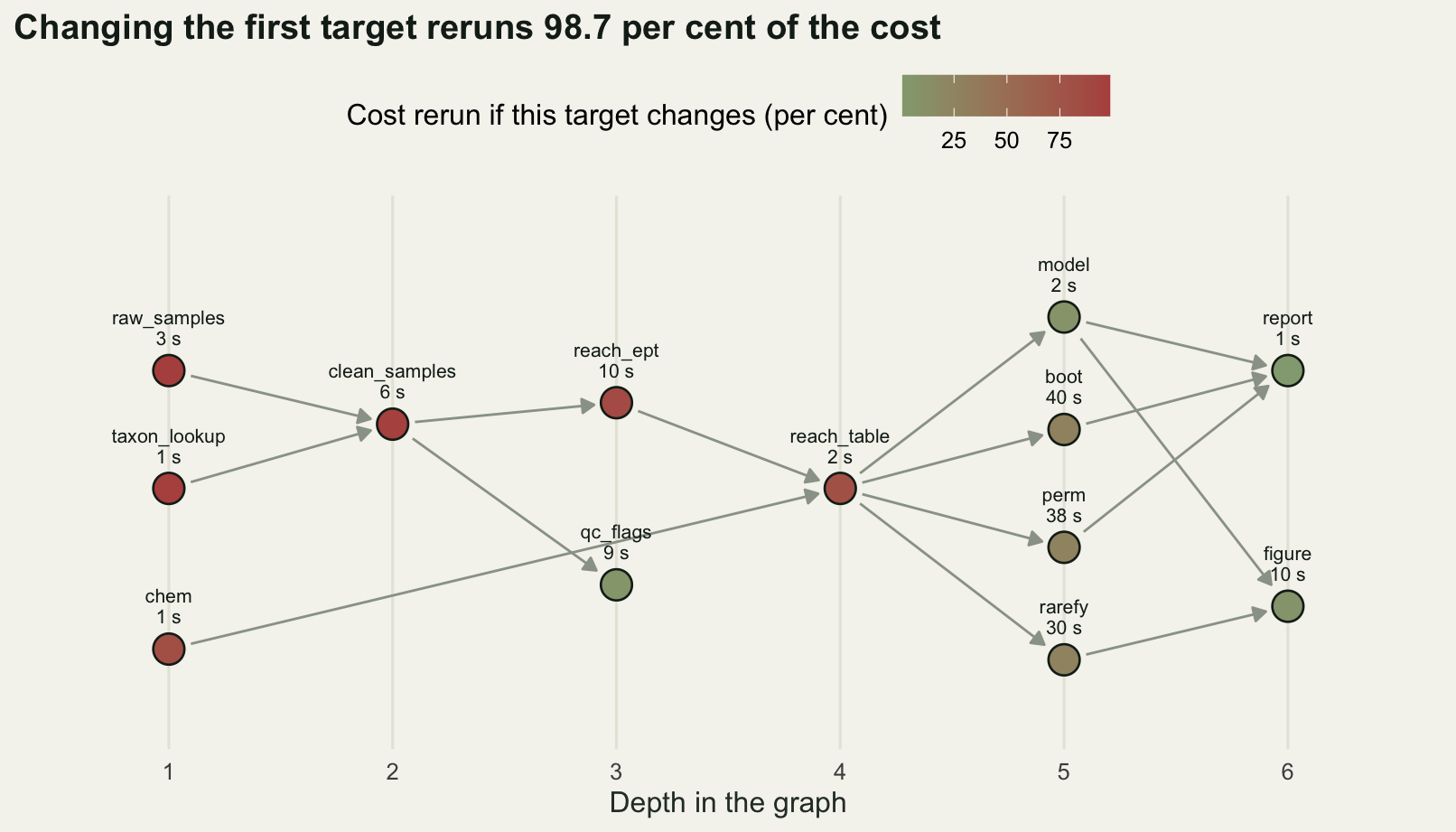
What one change makes stale
The propagator is the ten-line downstream function in the first chunk, the one that coloured the figure above. Given the set of targets you changed, walk forward along the edges until nothing new is reached. Everything reached is stale. Everything else is untouched and can keep its stored value.
That is the entire idea, and writing it out makes clear what it does not do. It does not know whether a target’s value would actually change; it knows that the target’s inputs changed, so its stored value is no longer a value anyone can vouch for. A pipeline is conservative in exactly this way, and the conservatism is the point: it never tells you that something is current when it is not.
stale_of <- function(changed) {
  d <- downstream(ed, changed)
  c(stale = length(d), cost = cost_of(d), percent = 100 * cost_of(d) / total_cost)
}

inval <- t(sapply(tg$target, function(n) stale_of(n)))
inval <- data.frame(target = rownames(inval), inval, row.names = NULL)
print(inval[order(-inval$percent), ])
target stale cost percent
1 raw_samples 11 151 98.6928105
2 taxon_lookup 11 149 97.3856209
4 clean_samples 10 148 96.7320261
6 reach_ept 8 133 86.9281046
3 chem 8 124 81.0457516
7 reach_table 7 123 80.3921569
9 boot 2 41 26.7973856
11 rarefy 2 40 26.1437908
10 perm 2 39 25.4901961
8 model 3 13 8.4967320
12 figure 1 10 6.5359477
5 qc_flags 1 9 5.8823529
13 report 1 1 0.6535948round(c(cheapest_change_percent = min(inval$percent),
dearest_change_percent = max(inval$percent),
median_change_percent = median(inval$percent),
targets_that_invalidate_over_half = sum(inval$percent > 50),
targets_that_invalidate_only_themselves = sum(inval$stale == 1)), 4) cheapest_change_percent dearest_change_percent
0.6536 98.6928
median_change_percent targets_that_invalidate_over_half
26.7974 6.0000
targets_that_invalidate_only_themselves
3.0000 The spread is the finding. Editing the taxon lookup, a small text table that maps recorded names to EPT membership, invalidates 97.3856 per cent of the pipeline’s cost. Editing the report, the last step, invalidates 0.6536 per cent: itself and nothing else. The median target invalidates 26.7974 per cent. There is no useful average here, because the values pile up at the two ends, with the inputs and the cleaning steps near the top and the outputs near the bottom. Which end your edit falls at is decided by the shape of the graph rather than by how big the edit felt.
Three of the thirteen targets invalidate only themselves. Those are the ones you can edit freely. The other ten cost something, and the dearest three to touch are the raw samples, the taxon lookup and the cleaning rule, which are the three a field season changes most often.
sl <- data.frame(
  target = factor(rep(inval$target, 2), levels = inval$target[order(inval$percent)]),
  value = c(inval$stale, inval$percent),
  lab = c(sprintf("%.0f", inval$stale), sprintf("%.1f", inval$percent)),
  share = rep(inval$percent, 2),
  panel = factor(rep(c("Targets made stale (count)",
                       "Share of total pipeline cost (per cent)"),
                     each = nrow(inval)),
                 levels = c("Targets made stale (count)",
                            "Share of total pipeline cost (per cent)")))

ggplot(sl, aes(value, target, fill = share)) +
  geom_col(width = 0.72) +
  geom_text(aes(label = lab), hjust = -0.15, size = 2.9, colour = te_pal$ink) +
  facet_wrap(~panel, scales = "free_x") +
  scale_fill_gradient(low = te_pal$sage, high = te_pal$clay,
                      name = "Cost rerun if this target changes (per cent)") +
  scale_x_continuous(expand = expansion(mult = c(0, 0.18)),
                     breaks = function(lims)
                       if (lims[2] < 20) seq(0, 10, by = 5) else seq(0, 90, by = 30)) +
  labs(x = NULL, y = NULL,
       title = "Six of the thirteen steps put over half the pipeline out of date") +
  theme_te() +
  theme(legend.position = "top",
        strip.text = element_text(colour = te_pal$ink, face = "bold", size = 9),
        panel.spacing.x = unit(1.6, "lines"),
        panel.grid.major.y = element_blank())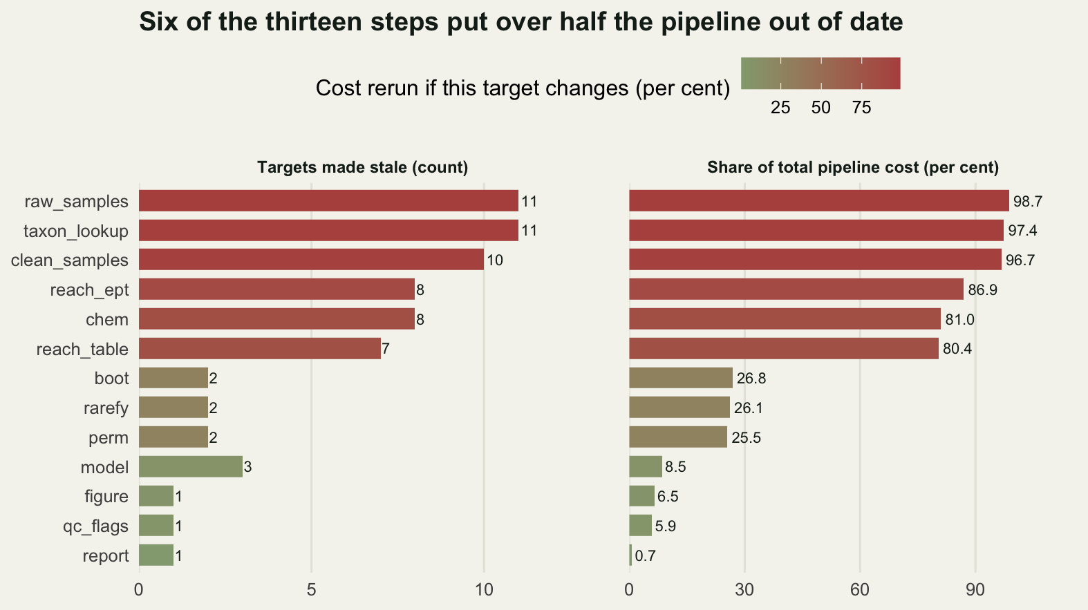
The analysis the targets actually run
Up to here the graph has been an abstraction with costs attached. To measure what a stale intermediate does to an ecological result, the targets have to compute something real. The data are simulated so that the pipeline can be rerun as many times as the measurement needs, and so that the correct answer at every stage is available for comparison.
Thirty reaches, forty taxa in the working list, three kick samples per reach. A taxon occurs at a reach with a probability that depends on how tolerant it is and how enriched the reach is, and the sensitive taxa are the ones on the EPT list, so EPT richness falls as phosphorus rises. Detection depends on how long the sample took, and nine samples were cut short.
set.seed(20260815)
n_pool <- 30
n_taxa <- 40
n_rep  <- 3

tp_pool <- round(exp(rnorm(n_pool, log(45), 0.85)), 1)
enrich  <- (log2(tp_pool) - min(log2(tp_pool))) /
  (max(log2(tp_pool)) - min(log2(tp_pool)))
tol <- c(sort(runif(22, 0, 0.62)), runif(18, 0.3, 1))
occ_p <- outer(enrich, tol, function(e, t) plogis(2.6 + 6.5 * (t - e)))
occ <- matrix(runif(n_pool * n_taxa) < occ_p, n_pool, n_taxa)

meta <- data.frame(
  reach  = rep(seq_len(n_pool), each = n_rep),
  rep    = rep(seq_len(n_rep), n_pool),
  effort = round(runif(n_pool * n_rep, 7, 12), 1))
short <- sample(nrow(meta), 9)
meta$effort[short] <- round(runif(9, 2, 4.6), 1)
det_p <- plogis(-1.4 + 0.30 * meta$effort)
obs <- matrix(FALSE, nrow(meta), n_taxa)
for (i in seq_len(nrow(meta)))
  obs[i, ] <- occ[meta$reach[i], ] & (runif(n_taxa) < det_p[i])

ept_v1 <- seq_len(n_taxa) <= 22
ept_v2 <- ept_v1
ept_v2[c(23, 24)] <- TRUE
ept_v2[22] <- FALSE

round(c(reaches_in_pool = n_pool, taxa = n_taxa, samples = nrow(meta),
        ept_taxa_lookup_v1 = sum(ept_v1), ept_taxa_lookup_v2 = sum(ept_v2),
        median_effort_minutes = median(meta$effort),
        shortened_samples = length(short),
        samples_in_the_first_build = sum(meta$reach <= 24),
        phosphorus_lowest = min(tp_pool), phosphorus_highest = max(tp_pool)), 4)
reaches_in_pool taxa
30.0 40.0
samples ept_taxa_lookup_v1
90.0 22.0
ept_taxa_lookup_v2 median_effort_minutes
23.0 9.3
shortened_samples samples_in_the_first_build
9.0 72.0
phosphorus_lowest phosphorus_highest
9.0 141.9 Each target is a function of the values its parents produced and of a list of settings. The settings are what the edits change: an effort threshold, which version of the taxon lookup is in force, whether the September batch is included, how richness is standardised, how many bootstrap replicates. Keeping them in one list is not tidiness for its own sake; it is what lets an edit be stated as a change to a named thing, which is what the propagator needs.
rec <- list()

rec$raw_samples <- function(v, p) {
  keep <- meta$reach <= p$n_reach & !(meta$reach %in% p$drop_reach)
  list(meta = meta[keep, ], obs = obs[keep, , drop = FALSE])
}
rec$taxon_lookup <- function(v, p) if (p$lookup == 1) ept_v1 else ept_v2
rec$chem <- function(v, p) {
  tp <- tp_pool[seq_len(p$n_reach)]
  if (p$chem_fix) tp[c(7, 19)] <- tp[c(7, 19)] * c(0.42, 0.55)
  data.frame(reach = seq_len(p$n_reach), tp = tp)
}
rec$clean_samples <- function(v, p) {
  r <- v$raw_samples
  keep <- r$meta$effort >= p$min_effort
  list(meta = r$meta[keep, ], obs = r$obs[keep, v$taxon_lookup, drop = FALSE])
}
rec$qc_flags <- function(v, p) {
  c(kept = nrow(v$clean_samples$meta),
    dropped = nrow(v$raw_samples$meta) - nrow(v$clean_samples$meta))
}
rec$reach_ept <- function(v, p) {
  cs <- v$clean_samples
  rs <- sort(unique(cs$meta$reach))
  val <- sapply(rs, function(r) {
    ix <- which(cs$meta$reach == r)
    if (p$standardise == "per_sample") mean(rowSums(cs$obs[ix, , drop = FALSE]))
    else sum(colSums(cs$obs[ix, , drop = FALSE]) > 0)
  })
  data.frame(reach = rs, ept = val)
}
rec$reach_table <- function(v, p) {
  m <- merge(v$reach_ept, v$chem, by = "reach")
  m$lp <- log2(m$tp)
  m
}
fit_it <- function(d) lm(ept ~ lp, data = d)
rec$model <- function(v, p) fit_it(v$reach_table)
rec$boot <- function(v, p) {
  d <- v$reach_table
  set.seed(p$boot_seed)
  s <- replicate(p$boot_reps, {
    ix <- sample(nrow(d), nrow(d), replace = TRUE)
    coef(fit_it(d[ix, ]))["lp"]
  })
  unname(quantile(s, c(0.025, 0.975)))
}
rec$perm <- function(v, p) {
  d <- v$reach_table
  set.seed(p$perm_seed)
  obs_slope <- coef(fit_it(d))["lp"]
  nul <- replicate(p$perm_reps, {
    dd <- d
    dd$lp <- sample(dd$lp)
    coef(fit_it(dd))["lp"]
  })
  unname((1 + sum(abs(nul) >= abs(obs_slope))) / (p$perm_reps + 1))
}
rec$rarefy <- function(v, p) round(mean(v$reach_table$ept), 4)
rec$figure <- function(v, p) c(points = nrow(v$reach_table), theme = p$fig_theme)
rec$report <- function(v, p)
  c(slope = unname(coef(v$model)["lp"]), lo = v$boot[1], hi = v$boot[2],
    p = v$perm)

settings <- list(n_reach = 24, drop_reach = integer(0), min_effort = 5,
                 lookup = 1, chem_fix = FALSE, standardise = "per_sample",
                 boot_reps = 400, boot_seed = 11, perm_reps = 400,
                 perm_seed = 12, fig_theme = 1)

build_all <- function(p) {
  v <- list()
  for (n in ord) v[[n]] <- rec[[n]](v, p)
  v
}
v0 <- build_all(settings)
round(v0$report, 4)
slope lo hi p
-4.4069 -4.9973 -3.8153 0.0025 print(v0$qc_flags) kept dropped
65 7 Two details in there are worth pausing on. The bootstrap sets its own seed from the settings rather than taking whatever state the session happens to be in, so its value depends only on its inputs and not on what ran before it; a target whose value depends on call order cannot be cached honestly. Checking an analysis script measures what happens when that rule is broken. And the report target does nothing except assemble four numbers other targets computed. That is deliberate: the thing the manuscript quotes should be a target, so that the question “is this current” has an answer.
The starting analysis reports 4.4069 EPT taxa lost per doubling of total phosphorus, with a bootstrap interval running from 3.8153 to 4.9973 taxa and a permutation p-value of 0.0025 against 400 shuffles. Seven of the 72 samples are dropped by the five-minute effort rule.
Three ways through the same fortnight of edits
Twelve edits, in the order they happened. Some are cosmetic, some change the data, one changes the definition of the response. Each edit is stated as a change to the settings plus the target or targets whose code or input it touches, which is the only thing the propagator needs to know.
edits <- list(
  list(lab = "figure axis relabelled",           tgt = "figure",
       set = list(fig_theme = 2)),
  list(lab = "effort threshold 5 to 8 minutes",  tgt = "clean_samples",
       set = list(min_effort = 8)),
  list(lab = "bootstrap 400 to 1200 draws",      tgt = "boot",
       set = list(boot_reps = 1200)),
  list(lab = "taxon lookup revised",             tgt = "taxon_lookup",
       set = list(lookup = 2)),
  list(lab = "September batch arrives",          tgt = c("raw_samples", "chem"),
       set = list(n_reach = 30)),
  list(lab = "phosphorus recalibrated",          tgt = "chem",
       set = list(chem_fix = TRUE)),
  list(lab = "richness pooled over replicates",  tgt = "reach_ept",
       set = list(standardise = "pooled")),
  list(lab = "permutation 400 to 1000 shuffles", tgt = "perm",
       set = list(perm_reps = 1000)),
  list(lab = "one reach excluded",               tgt = "raw_samples",
       set = list(drop_reach = 9L)),
  list(lab = "effort threshold back to 7",       tgt = "clean_samples",
       set = list(min_effort = 7)),
  list(lab = "second reach excluded",            tgt = "raw_samples",
       set = list(drop_reach = c(9L, 27L))),
  list(lab = "figure theme changed",             tgt = "figure",
       set = list(fig_theme = 3)))

mental <- ed[!(ed$from == "reach_table" & ed$to == "boot"), ]
mental <- rbind(mental, data.frame(from = "chem", to = "clean_samples"))

edit_cost <- t(sapply(edits, function(e)
  c(graph = cost_of(downstream(ed, e$tgt)),
    memory = cost_of(downstream(mental, e$tgt)),
    everything = total_cost)))
print(data.frame(edit = sapply(edits, function(e) e$lab), edit_cost))
edit graph memory everything
1 figure axis relabelled 10 10 153
2 effort threshold 5 to 8 minutes 148 108 153
3 bootstrap 400 to 1200 draws 41 41 153
4 taxon lookup revised 149 109 153
5 September batch arrives 152 112 153
6 phosphorus recalibrated 124 109 153
7 richness pooled over replicates 133 93 153
8 permutation 400 to 1000 shuffles 39 39 153
9 one reach excluded 151 111 153
10 effort threshold back to 7 148 108 153
11 second reach excluded 151 111 153
12 figure theme changed 10 10 153round(c(mean_cost_invalidated_per_edit_percent =
mean(100 * edit_cost[, "graph"] / total_cost),
edits_that_invalidate_over_half = sum(edit_cost[, "graph"] > total_cost / 2)), 4)mean_cost_invalidated_per_edit_percent edits_that_invalidate_over_half
68.4096 8.0000 The three strategies differ only in which targets they rebuild after each edit.
Rebuilding everything is the strategy that cannot be wrong. It runs all thirteen targets after every edit, including the thirty-second rarefaction that nothing upstream touched.
Letting the graph decide rebuilds the changed targets and everything downstream of them, in topological order.
The middle strategy is the one almost everyone actually uses: rebuild what you believe is affected. The analyst here is not careless. They have a mental model of the graph, and it is wrong in exactly two places. They believe the bootstrap reads the saved reach table from disk each time it runs, so they never think of it as needing a rebuild when the table changes; and they believe the cleaning step depends on the chemistry, so they rerun cleaning whenever a phosphorus value changes. One missing edge and one edge that does not exist.
run_sequence <- function(mode) {
  p <- settings
  v <- build_all(p)
  cost <- total_cost
  out <- data.frame(step = 0, cost = cost, rebuilt = length(ord),
                    slope = v$report[["slope"]], lo = v$report[["lo"]],
                    hi = v$report[["hi"]], pval = v$report[["p"]])
  for (k in seq_along(edits)) {
    e <- edits[[k]]
    for (nm in names(e$set)) p[[nm]] <- e$set[[nm]]
    hit <- switch(mode,
                  everything = tg$target,
                  graph = downstream(ed, e$tgt),
                  memory = downstream(mental, e$tgt))
    hit <- ord[ord %in% hit]
    for (n in hit) v[[n]] <- rec[[n]](v, p)
    cost <- cost + cost_of(hit)
    out <- rbind(out, data.frame(step = k, cost = cost, rebuilt = length(hit),
                                 slope = v$report[["slope"]],
                                 lo = v$report[["lo"]], hi = v$report[["hi"]],
                                 pval = v$report[["p"]]))
  }
  rownames(out) <- NULL
  out
}

truth_sequence <- function() {
  p <- settings
  v <- build_all(p)
  out <- data.frame(step = 0, slope = v$report[["slope"]], lo = v$report[["lo"]],
                    hi = v$report[["hi"]], pval = v$report[["p"]])
  for (k in seq_along(edits)) {
    for (nm in names(edits[[k]]$set)) p[[nm]] <- edits[[k]]$set[[nm]]
    v <- build_all(p)
    out <- rbind(out, data.frame(step = k, slope = v$report[["slope"]],
                                 lo = v$report[["lo"]], hi = v$report[["hi"]],
                                 pval = v$report[["p"]]))
  }
  rownames(out) <- NULL
  out
}

A <- run_sequence("everything")
G <- run_sequence("graph")
M <- run_sequence("memory")
TR <- truth_sequence()

agrees <- function(x) all(abs(x$slope - TR$slope) < 1e-9 &
                            abs(x$lo - TR$lo) < 1e-9 & abs(x$hi - TR$hi) < 1e-9)
round(c(cost_rebuild_everything = max(A$cost),
        cost_from_memory = max(M$cost),
        cost_let_the_graph_decide = max(G$cost),
        ratio_everything_over_graph = max(A$cost) / max(G$cost),
        ratio_memory_over_graph = max(M$cost) / max(G$cost),
        graph_saves_percent = 100 * (1 - max(G$cost) / max(A$cost)),
        memory_does_less_work_than_graph_percent =
          100 * (1 - max(M$cost) / max(G$cost)),
        target_rebuilds_everything = sum(A$rebuilt[-1]),
        target_rebuilds_graph = sum(G$rebuilt[-1]),
        target_rebuilds_memory = sum(M$rebuilt[-1])), 4)
cost_rebuild_everything
1989.0000
cost_from_memory
1114.0000
cost_let_the_graph_decide
1409.0000
ratio_everything_over_graph
1.4116
ratio_memory_over_graph
0.7906
graph_saves_percent
29.1604
memory_does_less_work_than_graph_percent
20.9368
target_rebuilds_everything
156.0000
target_rebuilds_graph
87.0000
target_rebuilds_memory
82.0000 c(rebuild_everything_matches_truth = agrees(A),
graph_matches_truth = agrees(G),
memory_matches_truth = agrees(M))rebuild_everything_matches_truth graph_matches_truth
TRUE TRUE
memory_matches_truth
FALSE Rebuilding everything costs 1989 declared seconds over the fortnight; letting the graph decide costs 1409, a saving of 29.1604 per cent. That is a real saving and it is smaller than the advertising suggests, because most of these edits are near the root of the graph and a root edit invalidates nearly everything. The average edit here invalidates 68.4096 per cent of the pipeline’s cost. A pipeline is not a way of making a badly shaped analysis cheap; it is a way of not paying for the parts that genuinely did not change.
The middle strategy costs 1114, which is 20.9368 per cent less work than the graph did. It is the cheapest of the three. It is also the only one whose reported numbers do not match a full rebuild, and that is the whole point of the comparison: the work it skipped was work that mattered.
wrong_ci <- abs(M$lo - TR$lo) > 1e-9 | abs(M$hi - TR$hi) > 1e-9
visible <- M$slope < M$lo | M$slope > M$hi
boot_due <- sapply(edits, function(e) "boot" %in% downstream(ed, e$tgt))
boot_run <- sapply(edits, function(e) "boot" %in% downstream(mental, e$tgt))

k <- nrow(M)
round(c(edits_after_which_the_estimate_was_wrong = sum(abs(M$slope - TR$slope) > 1e-9),
        edits_after_which_the_p_value_was_wrong = sum(abs(M$pval - TR$pval) > 1e-12),
        edits_after_which_the_interval_was_wrong = sum(wrong_ci),
        bootstrap_rebuilds_the_graph_would_have_run = sum(boot_due),
        bootstrap_rebuilds_the_analyst_ran = sum(boot_run),
        states_where_the_estimate_falls_outside_its_own_interval = sum(visible),
        wrong_states_with_no_visible_symptom = sum(wrong_ci) - sum(visible)), 4)
edits_after_which_the_estimate_was_wrong
0
edits_after_which_the_p_value_was_wrong
0
edits_after_which_the_interval_was_wrong
10
bootstrap_rebuilds_the_graph_would_have_run
9
bootstrap_rebuilds_the_analyst_ran
1
states_where_the_estimate_falls_outside_its_own_interval
6
wrong_states_with_no_visible_symptom
4 round(c(final_taxa_lost_per_doubling = -TR$slope[k],
correct_interval_low = -TR$hi[k], correct_interval_high = -TR$lo[k],
reported_interval_low = -M$hi[k], reported_interval_high = -M$lo[k],
correct_width = TR$hi[k] - TR$lo[k],
reported_width = M$hi[k] - M$lo[k],
low_end_understated_percent = 100 * (M$hi[k] - TR$hi[k]) / -TR$hi[k],
high_end_understated_percent = 100 * (M$lo[k] - TR$lo[k]) / -TR$lo[k],
overlap_of_the_two_intervals =
min(TR$hi[k], M$hi[k]) - max(TR$lo[k], M$lo[k]),
biggest_move_of_the_correct_interval_in_one_edit =
max(abs(diff(TR$lo)))), 4) final_taxa_lost_per_doubling
5.2095
correct_interval_low
4.5260
correct_interval_high
5.9688
reported_interval_low
3.7686
reported_interval_high
5.0756
correct_width
1.4428
reported_width
1.3071
low_end_understated_percent
16.7354
high_end_understated_percent
14.9645
overlap_of_the_two_intervals
0.5496
biggest_move_of_the_correct_interval_in_one_edit
1.0032 The estimate the analyst reports is right at every step, and so is the permutation p-value. Both of those targets sit in the part of the mental model that was correct, so they were rebuilt whenever they needed to be. The interval is wrong after 10 of the 12 edits.
The final numbers say it plainly. The correct interval for the loss of EPT taxa per doubling of phosphorus runs from 4.5260 to 5.9688 taxa, around an estimate of 5.2095. The reported interval runs from 3.7686 to 5.0756. On this run its low end is out by 16.7354 per cent and its high end by 14.9645 per cent, and the two intervals share 0.5496 taxa of width out of a correct width of 1.4428. Whatever the size of that gap, it is not noise. It is the interval from a data set that stopped existing nine edits ago, computed before the September reaches arrived, before the phosphorus recalibration, and before richness was redefined from a per-sample mean to a pooled count.
The graph would have rebuilt the bootstrap after 9 of the 12 edits. The analyst rebuilt it after 1, the one where they edited the bootstrap itself. Eight missed rebuilds, from a single wrong belief about one edge.
There is one symptom that is sometimes visible, and it is worth knowing about because it costs nothing to check. In 6 of the 13 states here the reported estimate falls outside its own reported interval, which is arithmetically impossible for a bootstrap of that estimate and is therefore proof that the two came from different runs. In the other 4 wrong states the estimate still sits inside the stale interval and nothing at all looks amiss. Comparing an estimate against its own interval is one line of code and it is the only warning the output itself can give you here.
lv <- c("Rebuild everything", "From memory", "Let the graph decide")
cost_df <- data.frame(
  step = rep(A$step, 3),
  value = c(A$cost, M$cost, G$cost),
  strategy = factor(rep(lv, each = nrow(A)), levels = lv),
  panel = "Cumulative rebuild cost (declared seconds)")
band_df <- data.frame(
  step = rep(A$step, 3),
  lo = -c(A$hi, M$hi, G$hi), hi = -c(A$lo, M$lo, G$lo),
  strategy = factor(rep(lv, each = nrow(A)), levels = lv),
  panel = "Reported EPT taxa lost per doubling of phosphorus")
est_df <- data.frame(step = A$step, value = -A$slope,
                     panel = "Reported EPT taxa lost per doubling of phosphorus")
pal3 <- c(te_pal$gold, te_pal$clay, te_pal$forest)

# the everything and graph bands hold identical values at every step, so the
# first is traced as an outline: three fills would paint over one another
band_fill <- band_df[band_df$strategy != "Rebuild everything", ]
band_edge <- band_df[band_df$strategy == "Rebuild everything", ]

ggplot(cost_df, aes(step, value)) +
  geom_ribbon(data = band_fill, aes(y = NULL, ymin = lo, ymax = hi, fill = strategy),
              alpha = 0.5) +
  geom_ribbon(data = band_edge, aes(y = NULL, ymin = lo, ymax = hi,
                                    colour = strategy),
              fill = NA, linetype = 2, linewidth = 0.6, show.legend = FALSE) +
  geom_line(data = est_df, aes(step, value), colour = te_pal$ink,
            linewidth = 0.9) +
  geom_point(data = est_df, aes(step, value), colour = te_pal$ink, size = 1.7) +
  geom_line(aes(colour = strategy), linewidth = 0.9) +
  geom_segment(data = data.frame(
    step = 5, value = 3.62,
    panel = "Reported EPT taxa lost per doubling of phosphorus"),
    aes(x = step, xend = step, y = value, yend = 4.2), colour = te_pal$ink,
    linewidth = 0.4) +
  geom_text(data = data.frame(
    step = 5, value = 3.48,
    panel = "Reported EPT taxa lost per doubling of phosphorus"),
    label = "reported estimate", size = 3.1, colour = te_pal$ink) +
  facet_wrap(~panel, ncol = 1, scales = "free_y") +
  scale_colour_manual(values = pal3, name = NULL, drop = FALSE) +
  scale_fill_manual(values = pal3, name = NULL, drop = FALSE, guide = "none") +
  scale_x_continuous(breaks = 0:12) +
  labs(x = "Edits made, in order",
       y = NULL,
       title = "The strategy that did the least work reported a nine-edit-old interval") +
  theme_te() +
  theme(legend.position = "top",
        strip.text = element_text(colour = te_pal$ink, face = "bold", size = 9))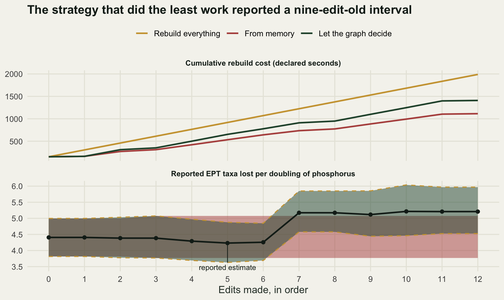
The lower panel is the shape worth remembering. The correct interval moves whenever the data or the definition move, in one case by 1.0032 taxa in a single edit, when richness changes from a per-sample mean to a count pooled across replicates: a shift of a sizeable fraction of the width of the interval itself. The reported interval moves once, early, and then holds still through seven substantive changes to the analysis. Nothing about the way it is displayed distinguishes the flat stretch from the moving one. It is a number in a caption, and it looks exactly like a number that was computed this morning.
Topological order and the parallel ceiling
The topological sort gives one valid order out of many. What it does not give is the shortest schedule, because targets with no path between them can run at the same time. The bound on that is the critical path: the longest chain of dependent targets, measured in cost. No amount of hardware gets you below it.
longest <- setNames(rep(NA_real_, nrow(tg)), tg$target)
for (n in ord) {
  p <- parents_of(ed, n)
  longest[n] <- tg$cost[tg$target == n] + if (length(p)) max(longest[p]) else 0
}
crit_len <- max(longest)
crit_path <- names(which.max(longest))
while (length(parents_of(ed, crit_path[1])) > 0) {
  p <- parents_of(ed, crit_path[1])
  crit_path <- c(p[which.max(longest[p])], crit_path)
}

makespan <- function(workers) {
  finish <- setNames(rep(NA_real_, nrow(tg)), tg$target)
  free <- rep(0, workers)
  left <- ord
  while (length(left) > 0) {
    ready <- left[sapply(left, function(n) all(!is.na(finish[parents_of(ed, n)])))]
    ready <- ready[order(-tg$cost[match(ready, tg$target)])]
    n <- ready[1]
    dep <- if (length(parents_of(ed, n))) max(finish[parents_of(ed, n)]) else 0
    w <- which.min(free)
    finish[n] <- max(free[w], dep) + tg$cost[tg$target == n]
    free[w] <- finish[n]
    left <- setdiff(left, n)
  }
  max(finish)
}

sched <- data.frame(workers = 1:6)
sched$makespan <- sapply(sched$workers, makespan)
sched$speedup <- total_cost / sched$makespan
print(round(sched, 4))
workers makespan speedup
1 1 153 1.0000
2 2 99 1.5455
3 3 63 2.4286
4 4 62 2.4677
5 5 62 2.4677
6 6 62 2.4677print(crit_path)[1] "raw_samples" "clean_samples" "reach_ept" "reach_table"
[5] "boot" "report" round(c(total_cost_seconds = total_cost,
critical_path_seconds = crit_len,
critical_path_targets = length(crit_path),
theoretical_ceiling = total_cost / crit_len,
speedup_at_three_workers = sched$speedup[3],
gain_from_a_fourth_worker = sched$speedup[4] - sched$speedup[3],
share_of_cost_on_the_critical_path = 100 * cost_of(crit_path) / total_cost,
ceiling_if_the_bootstrap_were_twice_as_fast =
(total_cost - 20) / (crit_len - 20)), 4) total_cost_seconds
153.0000
critical_path_seconds
62.0000
critical_path_targets
6.0000
theoretical_ceiling
2.4677
speedup_at_three_workers
2.4286
gain_from_a_fourth_worker
0.0392
share_of_cost_on_the_critical_path
40.5229
ceiling_if_the_bootstrap_were_twice_as_fast
3.1667 The critical path runs from the raw samples through cleaning, the richness summary, the reach table and the bootstrap to the report: 6 targets and 62 of the 153 declared seconds. The ceiling is therefore 2.4677, and the schedule reaches 2.4286 of that with three workers. A fourth worker adds 0.0392 and a fifth adds nothing at all.
ceiling_val <- total_cost / crit_len

ggplot(sched, aes(workers, speedup)) +
  geom_hline(yintercept = ceiling_val, linetype = 2, colour = te_pal$clay,
             linewidth = 0.8) +
  geom_line(colour = te_pal$forest, linewidth = 1) +
  geom_point(colour = te_pal$forest, size = 3.4) +
  geom_text(aes(label = sprintf("%.2f", speedup)), vjust = 1.9, size = 3.2,
            colour = te_pal$ink) +
  annotate("text", x = 3.5, y = ceiling_val + 0.11,
           label = sprintf("ceiling set by the critical path: %.4f", ceiling_val),
           size = 3.2, colour = te_pal$clay) +
  scale_x_continuous(breaks = 1:6) +
  scale_y_continuous(limits = c(0.75, 2.75)) +
  labs(x = "Workers running targets at the same time",
       y = "Speed-up over one worker",
       title = "A third worker is worth having and a fifth is worth nothing") +
  theme_te()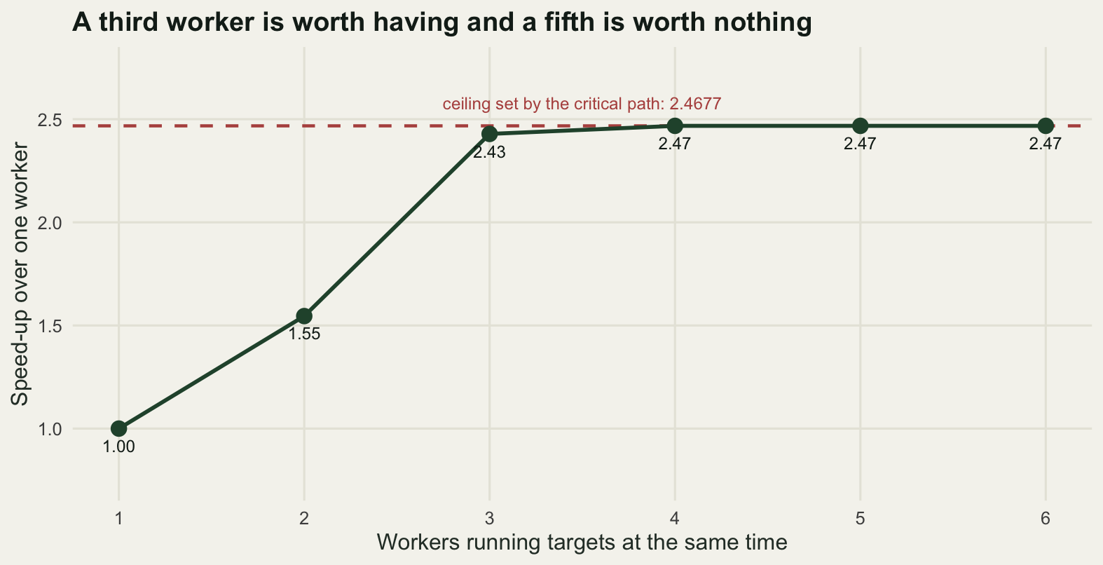
That ceiling is the useful thing to compute before buying anything, and it is a property of the graph rather than of the machine. A fourth core is worth 0.0392 here. Halving the bootstrap, which is on the critical path, raises the ceiling itself from 2.4677 to 3.1667, and it shortens the run on a single core as well, which no number of cores ever does. Working out which of your steps sit on the critical path is a loop over the topological order, and it tells you where an hour of programming pays and where it does not.
Two honest caveats about that ceiling. It assumes a worker is free the moment a target finishes and that moving a value between workers is free, neither of which is true; and it assumes the costs are right, which for a real pipeline means reading them off the log of a previous run rather than guessing.
What the targets package does with all this
Everything above is what the targets package does for you, with three differences that matter.
It works out the edges itself. You write the targets as function calls and it inspects the code to find which target names appear inside which expressions, so the edge list is derived from the analysis rather than maintained beside it. An edge list you maintain by hand goes stale in the same way a comment does.
It decides staleness by hashing rather than by timestamps. A target is out of date when the hash of its value’s inputs, the body of the function that made it, or its declared settings differ from what was recorded. That is stricter than the file modification times that make uses: touching a file without changing it does not trigger a rebuild, and changing a function body does, even though no file the target reads has changed. It is also the same idea as the lockfile in pinning package versions with renv: a recorded claim about the state something was built from.
And it stores the values, so tar_read(model) gives you the fitted model in a fresh session without running anything.
The pipeline lives in a file called _targets.R at the top of the project, and it is the same thirteen targets written in the package’s notation. It is not run here because this post has to render with nothing installed beyond ggplot2:
# _targets.R, read by the targets package
library(targets)
tar_option_set(packages = c("stats", "ggplot2"))
source("R/functions.R")

list(
  tar_target(raw_samples,   read_samples("data/kick_samples.csv")),
  tar_target(taxon_lookup,  read_lookup("data/ept_lookup.csv")),
  tar_target(chem,          read_chem("data/phosphorus.csv")),
  tar_target(clean_samples, clean_it(raw_samples, taxon_lookup, min_effort = 7)),
  tar_target(qc_flags,      count_dropped(raw_samples, clean_samples)),
  tar_target(reach_ept,     summarise_ept(clean_samples)),
  tar_target(reach_table,   join_reach(reach_ept, chem)),
  tar_target(model,         fit_it(reach_table)),
  tar_target(boot,          boot_ci(reach_table, reps = 1200, seed = 11)),
  tar_target(perm,          perm_test(reach_table, reps = 1000, seed = 12)),
  tar_target(rarefy,        rarefaction(reach_table)),
  tar_target(figure,        draw_it(reach_table, model, rarefy)),
  tar_target(report,        assemble(model, boot, perm))
)
Then four commands do the work of this entire post:
tar_outdated()     # which targets are stale, without running anything
tar_visnetwork()   # the graph, with the stale targets highlighted
tar_make()         # run exactly those, in topological order
tar_read(report)   # the value, without rerunning the pipeline
tar_outdated() is the one to run before you believe a number. It is the propagator from the second section, applied to the real analysis, and it answers the reviewer’s question in one line.
The idea is older than R. make has worked this way since 1976, Snakemake and Nextflow are the same graph with a different notation and a scheduler attached, and every one of them exists because the alternative is remembering.
The blog you are reading is an example
Quarto has this same machinery, narrowed to one file. Setting freeze: auto records the rendered output of each post and reruns a post’s R code only when that post’s source has changed:
execute:
  freeze: auto
This site runs on it, which is why editing one sentence in the About page does not rerun the simulations in the several hundred other posts.
n_posts <- 634
round(c(posts_on_this_site = n_posts,
        share_of_post_renders_a_one_post_edit_invalidates = 100 / n_posts,
        site_level_pages_downstream_of_every_post = 3), 4)
posts_on_this_site
634.0000
share_of_post_renders_a_one_post_edit_invalidates
0.1577
site_level_pages_downstream_of_every_post
3.0000 The arithmetic is the same as the second section of this post: editing one post invalidates 0.1577 per cent of the post renders. It is not the whole story, because the listing page, the sitemap and the feed are downstream of every post and are rebuilt each time, which is exactly the fan-in that the report target has in the graph above. The granularity of the freeze is the file, so a post with one cheap plot and a post with an hour of simulation in it are invalidated the same way, and moving that simulation out of the post and into a target of its own is what would make the granularity finer.
The honest limit
The graph only knows what you declared. That sentence is the limit, and the measurement above is a demonstration of it rather than an argument against it: the memory strategy failed because one edge was missing from the analyst’s model, and a pipeline tool fails in the same way when a dependency is invisible to it. A function that reads a file the pipeline does not know about, a global option set in a startup file, a package whose default changed under you, a value taken from the session’s random state: none of these are edges the tool can see, and each of them can change a result without making anything stale. That is the same failure the lockfile post is about, one level up.
Staleness is not correctness. Everything in this post measures whether the stored values are consistent with the current inputs and code. A pipeline that is entirely up to date can still be computing the wrong thing: the wrong model, the wrong exclusion rule, a units error of the kind testing your analysis code measures. The graph will faithfully rebuild a wrong answer and mark it current.
The three strategies were compared on one edit sequence, and the ratios depend on it. A fortnight in which the edits had all been cosmetic would show the graph saving far more than 29.1604 per cent, and a fortnight of nothing but data corrections would show it saving almost nothing. What does not depend on the sequence is the asymmetry: rebuilding too much wastes time, and rebuilding too little publishes numbers that came from different versions of the data. Only one of those two errors is visible in the output, and only 6 of the 10 wrong states here were visible even in principle.
The declared costs are stipulated, so every timing statement in the post is a ratio and none of it is a claim about wall clock seconds on any particular machine. And a pipeline has a cost of its own: the graph is code that has to be kept in step with the analysis, the stored values take disk space, and for a script that runs in four seconds and will never run again, all of this is overhead with no return. The threshold is roughly where the total rerun cost over the life of the project exceeds the cost of writing the graph down, which for an analysis rerun a dozen times with a bootstrap in it is crossed almost immediately, and for a one-afternoon calculation is never crossed at all.
Where to go next
The pipeline pins what is derived from what, and it says nothing about what the code was run with. That gap is the subject of pinning package versions with renv, where a changed default in a dependency moves the answer with no error and no warning, and of a reproducible statistical workflow in R, which is the wider argument this post is one part of.
If the ceiling calculation in the parallel section interested you, the thing to do before adding workers is to find out where the time is, which is what speeding up your analysis code measures, because the target on the critical path is usually not the one you expected. And once the graph exists, the functions inside the targets are ordinary functions with ordinary arguments, which makes them straightforward to test one at a time: testing your analysis code scores which kinds of test are worth writing.
References
Landau WM 2021 Journal of Open Source Software 6(57):2959 (10.21105/joss.02959)
Koster J, Rahmann S 2012 Bioinformatics 28(19):2520-2522 (10.1093/bioinformatics/bts480)
Di Tommaso P, Chatzou M, Floden EW, Prieto Barja P, Palumbo E, Notredame C 2017 Nature Biotechnology 35(4):316-319 (10.1038/nbt.3820)
Sandve GK, Nekrutenko A, Taylor J, Hovig E 2013 PLoS Computational Biology 9(10):e1003285 (10.1371/journal.pcbi.1003285)
Peng RD 2011 Science 334(6060):1226-1227 (10.1126/science.1213847)
Wilson G, Bryan J, Cranston K, Kitzes J, Nederbragt L, Teal TK 2017 PLoS Computational Biology 13(6):e1005510 (10.1371/journal.pcbi.1005510)