library(ggplot2)

te_pal <- list(forest = "#275139", green = "#2f8f63", sage = "#93a87f",
               clay = "#b5534e", gold = "#cda23f", line = "#dad9ca",
               ink = "#16241d", paper = "#f5f4ee")

theme_te <- function() {
  theme_minimal(base_size = 12) +
    theme(panel.grid.minor = element_blank(),
          panel.grid.major = element_line(colour = "#e7e6dc"),
          plot.background = element_rect(fill = "#f5f4ee", colour = NA),
          panel.background = element_rect(fill = "#f5f4ee", colour = NA),
          plot.title = element_text(face = "bold", colour = te_pal$ink),
          axis.title = element_text(colour = "#2c3a31"))
}Pinning package versions with renv
R
reproducibility
ecology tutorial
ggplot2
Build a lockfile by hand in base R, then measure what a quiet package update does to a reported ecological result: one tie-break rule, two different answers.
A manuscript comes back from review eleven months after it went out. One reviewer wants the dominance figure redrawn with the sites ordered by elevation, which is twenty minutes of work. You open the project folder, run the script, and it runs: no error, no warning, the figure appears in the plot pane looking much as it did. The number under it is not the number in the manuscript. The script has not been touched. The data file has not been touched. What has changed is the shelf of packages the script pulls its functions from, and nothing in the folder records what used to be on that shelf.
A lockfile is the record of what was on the shelf. It is a plain text file listing every package the project loaded, the exact version of each, where it came from, and a hash of the installed contents, and it is written on the day the analysis works. Read the other way round it is a claim: this result can be rebuilt, and here is the material list. The claim is worth exactly as much as the material list is complete, which is the subject of the last section of this post.
The machinery here is written by hand in base R, because the point is to see what a lockfile compares and what it cannot compare. An inventory is a data frame of four columns. A comparator is a match and a short stack of ifelse calls. What the real renv package adds is the part nobody wants to write: finding out what is installed, downloading exact versions from an archive, and keeping a per-project library so that two projects on the same machine can disagree about the version of vegan. Those calls appear here in blocks that are not run.
The measurement in the middle is the reason the post exists. One package changes one default between two releases: a rule for breaking ties, described in the release notes as an improvement, and it is an improvement. The analysis is a standard grassland one, and the reported result moves by an amount that no error message announces.
What a lockfile records
Four fields per package carry the whole idea. The name says which package. The version says which release. The source says which archive it came from, because a package installed from a GitHub branch and a package of the same name on CRAN are different software. The hash is a digest of the installed package, and it is the field that catches the case the version number misses.
The two inventories below are the state the manuscript was written from and the state of the library today. They are written out as literal data rather than read off this machine, partly because this post has to render anywhere, and partly because a constructed pair has a known answer to compare the comparator against. The version numbers are illustrative. The packages quadratkit and fieldnotes are invented; the rest are real names, and the versions attached to them here are not claims about those packages.
lock_a <- data.frame(
  package = c("MASS", "Matrix", "R6", "Rcpp", "cli", "digest", "ellipsis",
              "farver", "fieldnotes", "ggplot2", "glue", "gtable", "isoband",
              "labeling", "lattice", "lifecycle", "magrittr", "mgcv", "munsell",
              "nlme", "quadratkit", "rlang", "scales", "vegan"),
  version = c("7.3-60", "1.6-1", "2.5.1", "1.0.11", "3.6.2", "0.6.33", "0.3.2",
              "2.1.1", "0.3.1", "3.4.4", "1.6.2", "0.3.4", "0.2.7", "0.4.3",
              "0.21-8", "1.0.4", "2.0.3", "1.9-0", "0.5.0", "3.1-163", "1.4.2",
              "1.1.2", "1.3.0", "2.6-4"),
  source = c(rep("CRAN", 8), "GitHub", rep("CRAN", 15)),
  hash = c("0b1a1d", "9f7c02", "4e19aa", "c3d551", "77b0e4", "1ac9f8", "5d2b60",
           "8e4417", "a1c703", "62d9be", "3f8a15", "dd0c47", "7b6e92", "04ff3a",
           "e58d21", "b2470c", "6ca9d8", "39e1b5", "c07f4e", "aa3d16", "f19c8b",
           "2b6740", "90ec53", "51d8af"),
  stringsAsFactors = FALSE)

set_row <- function(d, pkg, ver, hsh) {
  i <- match(pkg, d$package)
  d$version[i] <- ver
  d$hash[i] <- hsh
  d
}

lock_b <- lock_a
lock_b <- set_row(lock_b, "quadratkit", "1.5.0", "7d40a2")
lock_b <- set_row(lock_b, "Matrix", "1.6-5", "e2b118")
lock_b <- set_row(lock_b, "mgcv", "1.9-1", "b4f206")
lock_b <- set_row(lock_b, "rlang", "1.1.3", "18cc7f")
lock_b <- set_row(lock_b, "fieldnotes", "0.3.1", "5e88d0")
lock_b <- lock_b[lock_b$package != "ellipsis", ]
lock_b <- rbind(lock_b, data.frame(package = "cpp11", version = "0.4.7",
                                   source = "CRAN", hash = "3a71ce"))
lock_b <- lock_b[order(lock_b$package), ]
rownames(lock_b) <- NULL

print(head(lock_a, 4))
package version source hash
1 MASS 7.3-60 CRAN 0b1a1d
2 Matrix 1.6-1 CRAN 9f7c02
3 R6 2.5.1 CRAN 4e19aa
4 Rcpp 1.0.11 CRAN c3d551c(packages_in_the_manuscript_state = nrow(lock_a),
packages_in_the_library_today = nrow(lock_b),
installed_from_github = sum(lock_a$source == "GitHub"))packages_in_the_manuscript_state packages_in_the_library_today
24 24
installed_from_github
1 The source field earns its place more often than people expect. Two packages can carry the same name and the same version string and be different software, and the usual way that happens in ecology is a package that lives on GitHub while its CRAN release lags behind, or a fork with one fix in it that somebody in the lab installed for a reason nobody wrote down. remotes::install_github leaves no trace in the library that says which commit you got. A record of the source is the difference between an instruction a stranger can follow and a name they have to guess at.
The hash is the field with the least obvious job and the most useful one. It is a digest of the package as installed, which means that two entries agree only if the contents agree, and it therefore catches every way a package can change without saying so: a reinstall from a moving branch, a rebuild against a different compiler, a local edit made in a hurry and forgotten. Version strings are written by people and hashes are computed from bytes, and only one of those two is reliable.
The real file is JSON rather than a data frame, and it carries a little more: the repositories the packages can be fetched from, the dependencies of each package, and the version of R that was running. The shape is the same.
{
  "R": { "Version": "4.3.3",
         "Repositories": [ { "Name": "CRAN", "URL": "https://cloud.r-project.org" } ] },
  "Packages": {
    "quadratkit": {
      "Package": "quadratkit",
      "Version": "1.4.2",
      "Source": "Repository",
      "Repository": "CRAN",
      "Hash": "f19c8b7e0d4a1c5b93e2f6087aa41d3c"
    }
  }
}
It is worth separating this file from the thing it is often confused with. A package’s DESCRIPTION carries a Depends field, and that field states a range: this package needs R at 4.3 or later and vegan at 2.6 or later. A range is what a package author wants, because a package has to work for everybody. A lockfile states a point: these exact versions, this hash. A point is what an analysis wants, because an analysis has to work once, on this data, and give the same answer when somebody checks it. The two coexist happily, and confusing them is how people end up believing that a package that declares its dependencies is a package whose results are reproducible.
Comparing two of these is a set operation on the package names followed by a field by field comparison of the packages both states hold. The order of the tests matters: a package that is only in one state is added or removed, and asking about its version first would compare a string with NA. A version that differs is reported as a version change, and only when the versions agree is the hash worth looking at, because a version change nearly always changes the hash as well and reporting both would be noise.
lock_diff <- function(a, b) {
  nm <- sort(union(a$package, b$package))
  ia <- match(nm, a$package)
  ib <- match(nm, b$package)
  va <- a$version[ia]; vb <- b$version[ib]
  ha <- a$hash[ia];    hb <- b$hash[ib]
  st <- ifelse(is.na(ia), "added",
        ifelse(is.na(ib), "removed",
        ifelse(va != vb, "version",
        ifelse(ha != hb, "hash only", "unchanged"))))
  data.frame(package = nm, from = va, to = vb, from_hash = ha, to_hash = hb,
             status = st, stringsAsFactors = FALSE)
}

bump_of <- function(from, to) {
  if (is.na(from) || is.na(to) || identical(from, to)) return(NA_character_)
  part <- function(v) as.integer(strsplit(v, "[.-]")[[1]])
  a <- part(from); b <- part(to)
  n <- max(length(a), length(b))
  a <- c(a, rep(0L, n - length(a)))
  b <- c(b, rep(0L, n - length(b)))
  c("major", "minor", "patch")[min(which(a != b)[1], 3)]
}

dif <- lock_diff(lock_a, lock_b)
moved <- dif[dif$status != "unchanged", ]
moved$bump <- mapply(bump_of, moved$from, moved$to)
rownames(moved) <- NULL

print(moved)
package from to from_hash to_hash status bump
1 cpp11 <NA> 0.4.7 <NA> 3a71ce added <NA>
2 ellipsis 0.3.2 <NA> 5d2b60 <NA> removed <NA>
3 fieldnotes 0.3.1 0.3.1 a1c703 5e88d0 hash only <NA>
4 Matrix 1.6-1 1.6-5 9f7c02 e2b118 version patch
5 mgcv 1.9-0 1.9-1 39e1b5 b4f206 version patch
6 quadratkit 1.4.2 1.5.0 f19c8b 7d40a2 version minor
7 rlang 1.1.2 1.1.3 2b6740 18cc7f version patchprint(table(dif$status))
    added hash only   removed unchanged   version
        1         1         1        18         4
cmp <- c(union_of_the_two_states = nrow(dif),
identical_in_both = sum(dif$status == "unchanged"),
differences = nrow(moved),
found_by_comparing_versions_only = sum(moved$status != "hash only"),
comparator_lines = length(deparse(lock_diff)) + length(deparse(bump_of)))
cmp union_of_the_two_states identical_in_both
25 18
differences found_by_comparing_versions_only
7 6
comparator_lines
27 The comparator is 27 lines as R deparses it, and on these two states it finds 7 differences against 18 packages that are identical in both. Four are version changes, one package has been added as an indirect dependency of something else, one has been dropped, and one has the same version string in both states with a different hash. That last row is the one to look at twice. It is the GitHub package: the version in its DESCRIPTION file was never bumped, the maintainer pushed new commits to the branch, and somebody reinstalled. Comparing versions alone finds 6 of the 7 differences and walks straight past it. This is the practical argument for the hash field, and it is why an inventory that records only names and versions is a weaker claim than it looks.
The bump column is the other thing worth noticing, and what it says is mostly negative. Three of the four version changes are patch releases, the sort that a maintainer publishes to fix a typo in a help page or a compiler warning. One is a minor release. Nothing about the size of the bump tells you whether the behaviour your analysis depends on has changed, because the numbering convention describes the maintainer’s intent about the interface, not the arithmetic underneath it. The next section is what happens when the intent and the arithmetic come apart.
The version that changed the answer
Twelve grassland sites, six grazed and six ungrazed, twenty quadrats at each, eight species counted in every quadrat. Solidago is the invasive of interest and grazing suppresses it, so the quantity the study reports is the percentage of quadrats in which Solidago is the most abundant species. Counts are Poisson with a site level and a quadrat level term, and because the underlying expected counts are kept, there is a true dominant species for every quadrat to compare against.
set.seed(20260814)
spp <- c("Achillea", "Bromus", "Dactylis", "Festuca",
         "Galium", "Lolium", "Plantago", "Solidago")
n_spec <- length(spp)
n_site <- 12
per_site <- 20
n_quad <- n_site * per_site
site <- rep(sprintf("S%02d", seq_len(n_site)), each = per_site)
treat <- rep(rep(c("grazed", "ungrazed"), each = per_site), n_site / 2)

base_lam <- c(1.5, 2.1, 1.8, 2.3, 1.3, 1.9, 1.4, 2.0)
lam <- matrix(rep(base_lam, each = n_quad), n_quad, n_spec)
lam[, n_spec] <- ifelse(treat == "ungrazed", 3.8, 1.0)
lam <- lam * exp(rnorm(n_site, 0, 0.2))[match(site, unique(site))] *
  exp(matrix(rnorm(n_quad * n_spec, 0, 0.6), n_quad, n_spec))
colnames(lam) <- spp
counts <- matrix(rpois(n_quad * n_spec, lam), n_quad, n_spec)
colnames(counts) <- spp
total_by_species <- colSums(counts)
tied <- apply(counts, 1, function(x) sum(x == max(x)) > 1)

print(counts[1:4, ])
Achillea Bromus Dactylis Festuca Galium Lolium Plantago Solidago
[1,] 3 0 0 1 0 1 1 0
[2,] 0 0 1 1 1 2 4 0
[3,] 1 3 2 4 0 0 3 3
[4,] 4 0 2 1 0 1 2 2print(total_by_species)Achillea Bromus Dactylis Festuca Galium Lolium Plantago Solidago
411 564 426 603 393 465 412 622 c(quadrats = n_quad, sites = n_site, quadrats_per_site = per_site,
species = n_spec, quadrats_with_a_tied_maximum = sum(tied)) quadrats sites
240 12
quadrats_per_site species
20 8
quadrats_with_a_tied_maximum
48 The counts are small, which is what a twenty by twenty centimetre quadrat in a species rich sward gives you, and small counts tie. In 48 of the 240 quadrats, 20 per cent of them, two or more species share the highest count. The data have no opinion about which of them is dominant. Some rule has to supply the answer, and the rule lives inside whichever function you call.
Here are the two versions of that function. Release 1.4.2 does what which.max does, which is to return the first position holding the maximum, so a tie goes to whichever species sits earliest in the column order. The columns arrived in alphabetical order from the field sheet, so in practice ties go to the species with the alphabetically earliest name. Release 1.5.0 changed this, and the release note reads: dominant() now resolves ties in favour of the species with the greater total abundance across the data set rather than by column position. That is a better rule. It is also silent, it needs no change to the calling script, and it appears in the interface as nothing at all.
dominant_142 <- function(cm, nm) nm[apply(cm, 1, which.max)]

dominant_150 <- function(cm, nm, weight) apply(cm, 1, function(x) {
  hit <- which(x == max(x))
  nm[hit[which.max(weight[hit])]]
})

dom_old <- dominant_142(counts, spp)
dom_new <- dominant_150(counts, spp, total_by_species)
dom_true <- spp[apply(lam, 1, which.max)]

share <- function(d, keep = rep(TRUE, n_quad)) 100 * mean(d[keep] == "Solidago")

round(c(tied_quadrats = sum(tied),
        tied_percent = 100 * mean(tied),
        quadrats_assigned_a_different_species = sum(dom_old != dom_new),
        of_those_untied = sum(dom_old != dom_new & !tied),
        reported_by_1_4_2 = share(dom_old),
        reported_by_1_5_0 = share(dom_new),
        percentage_points_gained = share(dom_new) - share(dom_old),
        relative_increase_percent = 100 * (share(dom_new) / share(dom_old) - 1),
        dominance_from_the_expected_counts = share(dom_true)), 4)
tied_quadrats tied_percent
48.0000 20.0000
quadrats_assigned_a_different_species of_those_untied
38.0000 0.0000
reported_by_1_4_2 reported_by_1_5_0
15.0000 23.7500
percentage_points_gained relative_increase_percent
8.7500 58.3333
dominance_from_the_expected_counts
22.9167 round(c(contrast_1_4_2 = share(dom_old, treat == "ungrazed") -
share(dom_old, treat == "grazed"),
contrast_1_5_0 = share(dom_new, treat == "ungrazed") -
share(dom_new, treat == "grazed"),
contrast_from_expected_counts = share(dom_true, treat == "ungrazed") -
share(dom_true, treat == "grazed"),
quadrats_right_1_4_2_percent = 100 * mean(dom_old == dom_true),
quadrats_right_1_5_0_percent = 100 * mean(dom_new == dom_true),
ties_resolved_correctly_1_4_2 = sum(dom_old[tied] == dom_true[tied]),
ties_resolved_correctly_1_5_0 = sum(dom_new[tied] == dom_true[tied])), 4) contrast_1_4_2 contrast_1_5_0
25.0000 29.1667
contrast_from_expected_counts quadrats_right_1_4_2_percent
40.8333 51.2500
quadrats_right_1_5_0_percent ties_resolved_correctly_1_4_2
54.1667 11.0000
ties_resolved_correctly_1_5_0
18.0000 site_old <- 100 * tapply(dom_old == "Solidago", site, mean)
site_new <- 100 * tapply(dom_new == "Solidago", site, mean)
print(rbind(reported_by_1_4_2 = site_old, reported_by_1_5_0 = site_new)) S01 S02 S03 S04 S05 S06 S07 S08 S09 S10 S11 S12
reported_by_1_4_2 5 45 0 40 0 15 0 30 0 20 10 15
reported_by_1_5_0 15 60 5 40 15 30 5 30 0 30 15 40round(c(sites_that_move = sum(site_old != site_new),
largest_site_shift = max(abs(site_new - site_old)),
sites_changing_rank = sum(rank(-site_old, ties.method = "min") !=
rank(-site_new, ties.method = "min"))), 4) sites_that_move largest_site_shift sites_changing_rank
9 25 8 lev <- c("quadratkit 1.4.2", "quadratkit 1.5.0")
ord <- names(sort(site_old + 0.001 * site_new))
dom_df <- data.frame(
site = factor(rep(names(site_old), 2), levels = ord),
value = c(as.numeric(site_old), as.numeric(site_new)),
release = factor(rep(lev, each = n_site), levels = lev))
seg_df <- data.frame(site = factor(names(site_old), levels = ord),
lo = as.numeric(site_old), hi = as.numeric(site_new))
ggplot(dom_df, aes(value, site)) +
geom_segment(data = seg_df, aes(x = lo, xend = hi, y = site, yend = site),
inherit.aes = FALSE, colour = te_pal$line, linewidth = 2.6) +
geom_vline(xintercept = share(dom_old), colour = te_pal$forest,
linetype = "22", linewidth = 0.6) +
geom_vline(xintercept = share(dom_new), colour = te_pal$clay,
linetype = "22", linewidth = 0.6) +
geom_point(aes(shape = release, colour = release), size = 3.3, stroke = 1.1) +
scale_shape_manual(values = c(1, 16), name = NULL) +
scale_colour_manual(values = c(te_pal$forest, te_pal$clay), name = NULL) +
scale_x_continuous(limits = c(-2, 64), breaks = seq(0, 60, by = 10)) +
labs(x = "Quadrats dominated by Solidago (per cent)", y = NULL,
title = "The same counts, two releases, nine sites with a different answer",
subtitle = "quadratkit is an invented package; the quadrat counts are simulated") +
theme_te() +
theme(legend.position = "top")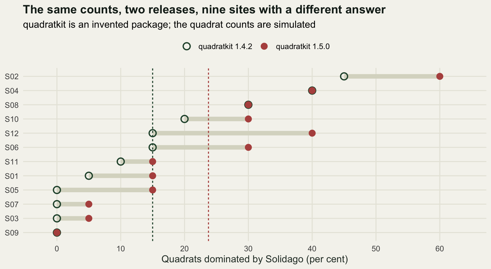
quadratkit is an invented package and its two release numbers are illustrative; no real package behaves this way. The bar joining each pair of points is the amount the reported value moved. The two vertical lines are the whole survey figures the two releases give, 15 per cent and 23.75 per cent.
The survey wide figure the script reports moves from 15 per cent under 1.4.2 to 23.75 per cent under 1.5.0. That is 8.75 percentage points, and it is a relative change of 58.3333 per cent: the newer release reports the invasive as dominant in more than one and a half times as many quadrats. The grazing contrast, the difference between the ungrazed and the grazed sites, moves from 25 to 29.1667 percentage points. At the site level 9 of the 12 sites report a different value, the largest single site moving by 25 percentage points, and 8 of the 12 sites change their rank, which matters because the site ranking is what a management report is usually built on.
There are three ways a package update can reach you, and they are not equally expensive. A function that has been removed or an argument that has been renamed stops the script where it stands, which is the cheapest possible outcome: the error message names the call, and half an hour of reading a changelog fixes it. A deprecation warning is nearly as good, because it prints, and because it usually arrives one release before the behaviour actually changes, which is the whole purpose of the convention. The third way is the one in this section. The interface is untouched, no condition is signalled, the script runs to the end, and the only evidence that anything happened is a number that does not match a number written down elsewhere. Whether you notice depends entirely on whether you still have the old number and whether you bother to compare.
Nothing raised a condition here. The function has the same name, takes the same arguments, and returns a character vector of the same length. Every check in checking an analysis script passes on both runs, because each run is internally consistent: it runs from a clean session, it gives the same answer twice, and it survives a row shuffle. The two runs are consistent with each other about everything except the answer.
The uncomfortable part is that 1.5.0 is right. Compared against the species with the highest expected count in each quadrat, the new rule is correct in 54.1667 per cent of quadrats against 51.25 per cent for the old one, and among the 48 tied quadrats it picks the true dominant 18 times against 11. Its survey wide figure of 23.75 per cent sits close to the 22.9167 per cent the expected counts give, while the old rule’s 15 per cent is a long way below. The old rule was biased, because giving every tie to the alphabetically earliest species takes ties away from Solidago systematically, and Solidago is last in the alphabet here. The upgrade fixed a real defect.
None of which helps the manuscript. The published figure says 15 per cent, the reviewer will be sent a figure saying 23.75 per cent, and the difference has to be explained in a letter. The value of the lockfile is not that it keeps you on the old version forever. It is that it lets you produce the old number on demand, see that the difference is 8.75 points, find out why in an afternoon rather than a fortnight, and then decide, in the open, to move to the better rule and reprint the figure.
Finding the line that did it
Without an inventory the search space is the whole library: every package that was installed then and is installed now, at whatever version each happens to be. With the two states and the comparator, the space is the 7 packages that differ. One more filter is nearly free: most of those packages are indirect dependencies the script never mentions, so scan the script text for library() calls and for names qualified with a double colon, and intersect.
script_src <- c(
  "library(ggplot2)",
  "library(vegan)",
  "library(quadratkit)",
  "notes  <- fieldnotes::read_field_notes('quadrats-2019.txt')",
  "counts <- quadratkit::as_quadrat_matrix(notes)",
  "dom    <- quadratkit::dominant(counts)",
  "share  <- 100 * mean(dom == 'Solidago')",
  "shan   <- vegan::diversity(counts)",
  "fit    <- mgcv::gam(share ~ s(elevation), data = env)",
  "ggplot(env, aes(elevation, share)) + geom_point()")

packages_named <- function(src) {
  qualified <- gregexpr("[A-Za-z][A-Za-z0-9.]*(?=::)", src, perl = TRUE)
  attached <- gregexpr("(?<=library\\()[A-Za-z][A-Za-z0-9.]*", src, perl = TRUE)
  sort(unique(c(unlist(regmatches(src, qualified)),
                unlist(regmatches(src, attached)))))
}

named <- packages_named(script_src)
suspects <- intersect(moved$package, named)
print(named)
[1] "fieldnotes" "ggplot2" "mgcv" "quadratkit" "vegan" print(suspects)[1] "fieldnotes" "mgcv" "quadratkit"c(packages_in_the_union = nrow(dif),
packages_that_differ = nrow(moved),
packages_the_script_names = length(named),
differ_and_named = length(suspects),
halvings_over_the_whole_library = ceiling(log2(nrow(dif))),
halvings_over_the_suspects = ceiling(log2(length(suspects)))) packages_in_the_union packages_that_differ
25 7
packages_the_script_names differ_and_named
5 3
halvings_over_the_whole_library halvings_over_the_suspects
5 2 print(table(tie = tied, changed = dom_old != dom_new)) changed
tie FALSE TRUE
FALSE 192 0
TRUE 10 38c(untied_quadrats_that_changed = sum(!tied & dom_old != dom_new),
tied_quadrats_that_changed = sum(tied & dom_old != dom_new),
tied_quadrats_left_alone = sum(tied & dom_old == dom_new))untied_quadrats_that_changed tied_quadrats_that_changed
0 38
tied_quadrats_left_alone
10 Two filters and the search is nearly over. The union of the two states holds 25 packages; 7 of them differ; 5 are named by the script; 3 are in both sets. Downgrading half of the candidates at a time and rerunning is a binary search, so the difference between the two search spaces is 5 halvings against 2: an afternoon against a coffee break. The three surviving suspects are quadratkit, fieldnotes whose hash moved without its version changing, and mgcv, whose smoother is fitted after the reported percentage has already been computed.
The confirmation is in the cross tabulation, and it is worth more than the narrowing. Of the 240 quadrats, 0 of the untied ones were assigned a different species by the two releases, and all 38 changes sit among the 48 tied quadrats. If the discrepancy came from anywhere other than the tie rule, untied quadrats would move too. That single table takes the diagnosis from a plausible story to a checked one, and it is the shape of confirmation to look for whenever a version change is the suspect: find the subset of the data the changed rule can touch, and show that nothing outside it moved.
The mechanics of the search are worth spelling out, because the obvious way to do it is the wrong one. Do not downgrade packages in your main library: install the candidate version into a scratch library, point the session at it, run the analysis, and record the number. renv gives you this for free, since the project library is already separate from everything else, and the whole operation is renv::install("quadratkit@1.4.2") followed by a rerun and then renv::restore() to put the project back where it was. What you are looking for at each step is not whether the script runs. It is whether the reported number moves, so the comparison has to be against a number you wrote down before you started, which is the argument for printing the quantities that matter rather than only plotting them.
Sometimes the old version cannot be reinstalled at all. A package that has been removed from CRAN keeps its archived source tarballs, so the version is usually still fetchable and simply has to be compiled, which for anything with C or Fortran in it means a working toolchain and occasionally a compiler that no longer accepts the code. A package installed from a branch that has since been force-pushed or deleted is gone, and the hash in the lockfile then serves only as evidence of what you had. This asymmetry is a good reason to prefer an archived source for anything a published result rests on, and to treat a GitHub dependency as a temporary state rather than a permanent one.
step_lab <- c("In the library, either state",
              "Differ between the two states",
              "Differ and named by the script",
              "Accounts for every changed quadrat")
narrow_df <- data.frame(
  step = factor(step_lab, levels = rev(step_lab)),
  n = c(nrow(dif), nrow(moved), length(suspects), 1))

ggplot(narrow_df, aes(n, step)) +
  geom_col(fill = te_pal$forest, width = 0.6) +
  geom_text(aes(label = n), hjust = -0.4, colour = te_pal$ink, size = 4) +
  scale_x_continuous(limits = c(0, 28), breaks = seq(0, 25, by = 5)) +
  labs(x = "Packages still under suspicion", y = NULL,
       title = "Two cheap filters take a 25 way search down to 3") +
  theme_te()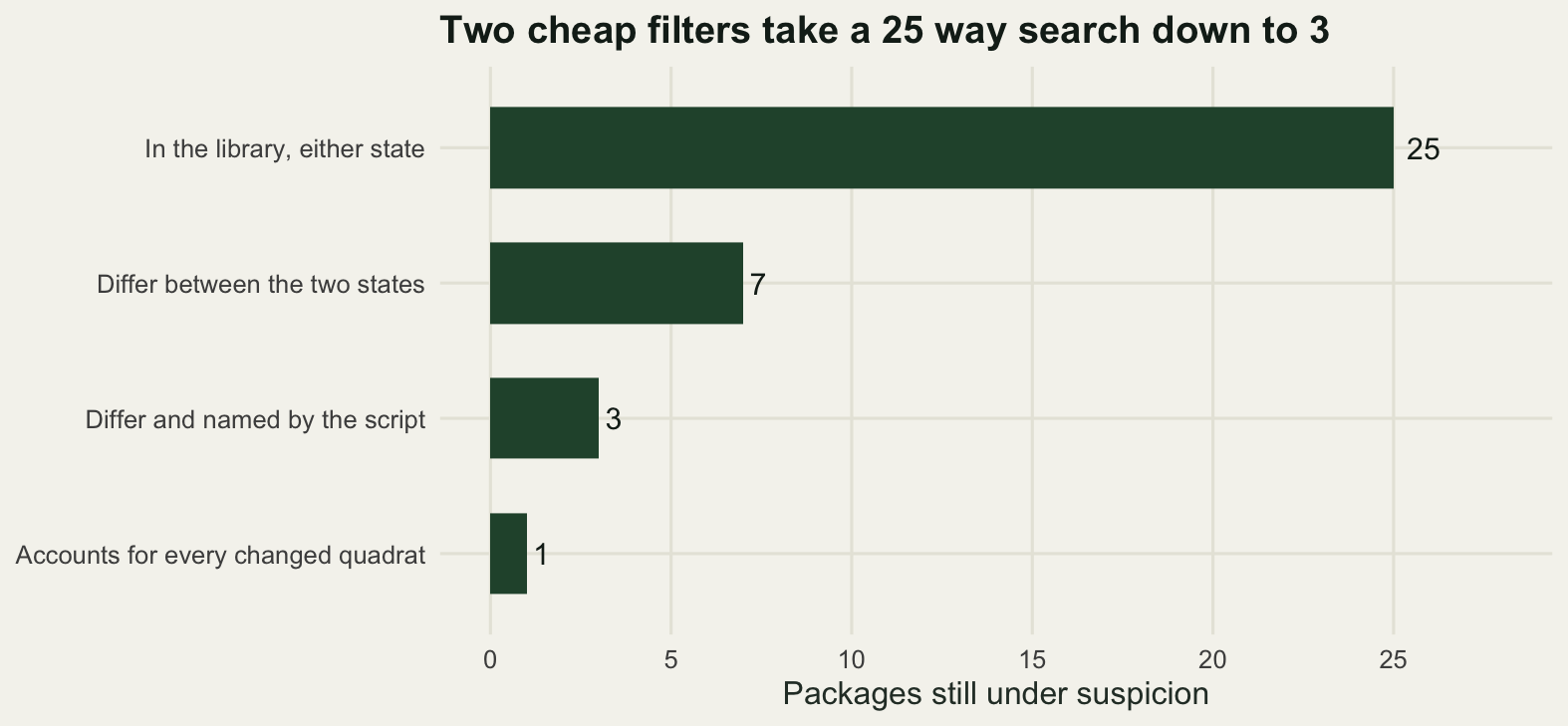
Ties are a function of counting effort
The size of the discrepancy is not a property of the package. It is a property of the data, and specifically of how many quadrats have a tied maximum, which falls as counts get larger. That makes the exposure of an analysis to this class of change something you can estimate before it bites: count the ties.
The sweep below multiplies the expected counts by a factor from a quarter to eight, which is what happens when you use a larger quadrat, count for longer, or pool two visits. At each level 80 independent count matrices are drawn from the same expected values, and both releases are run on each.
set.seed(20260814)
effort <- c(0.25, 0.5, 1, 2, 4, 8)
n_rep <- 80
sweep <- t(sapply(effort, function(e) {
  rep_out <- t(replicate(n_rep, {
    cm <- matrix(rpois(n_quad * n_spec, lam * e), n_quad, n_spec)
    tt <- colSums(cm)
    c(tie = 100 * mean(apply(cm, 1, function(x) sum(x == max(x)) > 1)),
      old = share(dominant_142(cm, spp)),
      new = share(dominant_150(cm, spp, tt)),
      mean_count = mean(cm))
  }))
  colMeans(rep_out)
}))
sweep <- cbind(effort = effort, sweep, gap = sweep[, "new"] - sweep[, "old"])
gap_share <- sweep[, "gap"] / sweep[, "tie"]
lo <- 1
hi <- nrow(sweep)
print(round(sweep, 4))
effort tie old new mean_count gap
[1,] 0.25 43.9479 10.4583 22.0156 0.5066 11.5573
[2,] 0.50 32.5990 13.5104 22.1042 1.0100 8.5937
[3,] 1.00 22.3594 16.5521 22.5313 2.0132 5.9792
[4,] 2.00 13.5833 18.6250 22.1875 4.0480 3.5625
[5,] 4.00 7.5833 20.5885 22.3854 8.0900 1.7969
[6,] 8.00 4.2187 21.4635 22.4948 16.1745 1.0313eff_sum <- round(c(replicates_at_each_level = n_rep,
tie_rate_at_the_lowest_effort = unname(sweep[lo, "tie"]),
tie_rate_at_the_highest_effort = unname(sweep[hi, "tie"]),
gap_at_the_lowest_effort = unname(sweep[lo, "gap"]),
gap_at_the_highest_effort = unname(sweep[hi, "gap"]),
old_rule_at_the_lowest_effort = unname(sweep[lo, "old"]),
old_rule_at_the_highest_effort = unname(sweep[hi, "old"]),
new_rule_at_its_lowest = min(sweep[, "new"]),
new_rule_at_its_highest = max(sweep[, "new"]),
smallest_gap_as_a_share_of_the_tie_rate = min(gap_share),
largest_gap_as_a_share_of_the_tie_rate = max(gap_share),
target_from_the_expected_counts = share(dom_true)), 4)
eff_sum replicates_at_each_level tie_rate_at_the_lowest_effort
80.0000 43.9479
tie_rate_at_the_highest_effort gap_at_the_lowest_effort
4.2187 11.5573
gap_at_the_highest_effort old_rule_at_the_lowest_effort
1.0313 10.4583
old_rule_at_the_highest_effort new_rule_at_its_lowest
21.4635 22.0156
new_rule_at_its_highest smallest_gap_as_a_share_of_the_tie_rate
22.5313 0.2370
largest_gap_as_a_share_of_the_tie_rate target_from_the_expected_counts
0.2674 22.9167 ser <- c("Quadrats with a tied maximum", "Reported by 1.4.2",
"Reported by 1.5.0")
eff_df <- data.frame(
mean_count = rep(sweep[, "mean_count"], 3),
value = c(sweep[, "tie"], sweep[, "old"], sweep[, "new"]),
series = factor(rep(ser, each = nrow(sweep)), levels = ser))
ref_val <- share(dom_true)
ref_lab <- sprintf("Reference: %.4f per cent, from the expected counts", ref_val)
ggplot(eff_df, aes(mean_count, value, colour = series)) +
geom_hline(yintercept = ref_val, linetype = "12", colour = te_pal$ink,
linewidth = 0.45) +
annotate("text", x = 2.35, y = 28.8, label = ref_lab, hjust = 0, size = 3.5,
colour = te_pal$ink) +
annotate("segment", x = 2.6, xend = 2.6, y = 27.4, yend = 23.5,
colour = te_pal$ink, linewidth = 0.35) +
geom_line(linewidth = 1) +
geom_point(size = 2.6) +
scale_colour_manual(values = c(te_pal$gold, te_pal$forest, te_pal$clay),
name = NULL) +
scale_x_continuous(transform = "log2", breaks = c(0.5, 1, 2, 4, 8, 16)) +
scale_y_continuous(limits = c(0, 50)) +
guides(colour = guide_legend(nrow = 1)) +
labs(x = "Mean count per species per quadrat",
y = "Per cent of quadrats",
title = "The gap between the releases is about a quarter of the tie rate") +
theme_te() +
theme(legend.position = "top")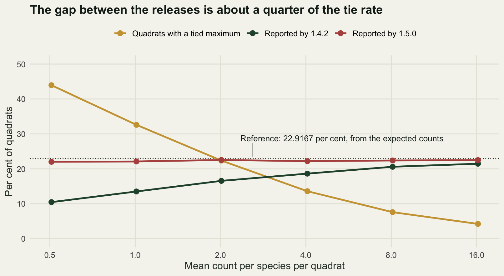
At a quarter of the original effort, mean counts near a half per species per quadrat, 43.9479 per cent of quadrats are tied and the two releases differ by 11.5573 percentage points. At eight times the original effort the tie rate is 4.2187 per cent and they differ by 1.0313. The older release is the one that moves: its reported dominance climbs from 10.4583 to 21.4635 per cent as counts grow, while the newer one sits between 22.0156 and 22.5313 throughout, close to the 22.9167 per cent the expected counts imply at every level of effort.
The tie rate is the ceiling on the disagreement rather than the disagreement itself, and the sweep says how far below that ceiling it sits: the gap runs between 0.237 and 0.2674 of the tie rate across the six effort levels. Counting the ties gives you the bound directly, and dividing it by four gives you the exposure. What holds steady is the fraction and not the difference, because the two rules part company on the reported figure only over the quadrats where Solidago is among the species level at the top, and how often that happens is a property of the community rather than of how hard anybody counted.
There are two readings of that, and both are useful. The narrow one is about version pinning: a survey with small counts is much more exposed to a change in a tie rule than a survey with large ones, so the same package update that moves a well counted survey by one percentage point moves a thinly counted one by eleven. The wide reading is about the study design, and it does not need a package at all. Reporting the single most abundant species per quadrat throws away the information that two species were level, which at the counts in this survey is a fifth of the quadrats and at a quarter of the effort more than two fifths of them. A summary that reports the tie honestly, whether as a shared dominance or as a missing value, would have been immune to the whole episode. When a package’s tie-break rule can move your headline number by 8.75 points, the number was resting on a convention, not on the counts.
What a tie-honest summary looks like depends on the question. If the point is which species holds the quadrat, then a tied quadrat has no answer and the honest value is a missing one, counted and reported: NA in 48 of 240 quadrats is a statement about the survey rather than about the software. If the point is the invasive’s importance, the count itself is a better quantity than the rank derived from it, and a mean relative abundance never ties. If the dominance classification is genuinely what the management report needs, then the tie rule belongs in the methods section of the paper, written out in a sentence, which also means somebody has to decide it deliberately once instead of inheriting it from an argument default. Any of the three would have made this post’s measurement impossible, which is the strongest thing that can be said for them.
Using renv for real
Everything above is the model of what renv does; this is what you type. Four calls cover most of the working life of a project. They are not run here because this post has to render with nothing installed beyond ggplot2.
# once, in the project directory
renv::init()      # private library for this project, plus renv.lock and .Rprofile

# after installing or updating anything the analysis needs
renv::snapshot()  # rewrite renv.lock from what is currently loaded

# on another machine, or on yours in eleven months
renv::restore()   # install exactly what renv.lock names

# at any time
renv::status()    # what the library and the lockfile disagree about
init() writes three things: a project library under renv/library, the lockfile renv.lock, and a one line .Rprofile that points R at the project library whenever the project is opened. That last file is what makes the arrangement work without any discipline from you, and it is also why the first sign that renv is installed on a project is usually that install.packages starts putting things somewhere new.
snapshot() is the one to be deliberate about. By default it records the packages your project code actually uses, found by scanning your sources the way packages_named does above, rather than everything in the library. Run it when the analysis works, not when you are halfway through installing things, and commit renv.lock alongside the script it belongs to. A lockfile that is not under version control is a note to yourself; a lockfile committed next to the script is a claim anybody can check, which is the argument git for ecologists makes about everything else in the project folder.
restore() is the claim being cashed. It reads the lockfile and installs those exact versions into the project library, from CRAN’s archive for packages that are no longer current, and from the recorded commit for packages installed off GitHub. It does not touch the rest of your machine.
status() is the one to run before you believe a result. It compares the library against the lockfile and tells you which packages have drifted, which is the same comparison as lock_diff above, run against the live library instead of a second lockfile.
There is a fifth call worth knowing, renv::update(), and the reason to name it is that it is the one that should be done on purpose. Update between projects, or at the start of a piece of work, never in the middle of a revision. Then run the analysis, compare the numbers with the ones you had, and snapshot only when you have looked at the difference.
The cost side is real and small, and it is worth knowing before you meet it rather than in the middle of a deadline. A project library is a second copy of everything, so a machine with six renv projects on it holds six copies of ggplot2 unless the cache is doing its job, which by default it is: renv keeps one copy of each package version under a global cache and links the project libraries to it, so the disk cost of a new project that uses versions you already have is close to nothing. The time cost lands on the first restore() on a new machine, and on Linux it lands hard, because CRAN supplies source rather than binaries there and a package such as sf or Matrix has to be compiled. Budget an afternoon for the first restore of a large project on a fresh Linux box, and a couple of minutes for the same operation on a machine that already has the cache warm.
Two situations catch people out. On a shared cluster, the project library sits inside the project directory, which is often on a network filesystem with a quota, and the sensible arrangement is to put the cache somewhere local and roomy. And when a project renders with Quarto, the R session Quarto starts has to be the one that sees the project library, which it will be if the render runs from the project directory so that the .Rprofile is read: rendering from somewhere else quietly uses the system library instead, and the whole arrangement is silently switched off.
How often does drift matter? That depends on a rate nobody has measured for the packages an ecologist uses, so the block below is arithmetic on an assumed rate rather than a measurement of one. Give each package an independent probability per year of a release that changes some behaviour an analysis might rest on, and ask for the chance that at least one of the 24 packages does so.
rate <- c(0.02, 0.05, 0.10)
years <- c(1, 3, 5)
drift <- outer(rate, years, function(p, y) 100 * (1 - (1 - p)^(nrow(lock_a) * y)))
dimnames(drift) <- list(sprintf("rate %.2f", rate), sprintf("%d yr", years))
drift <- round(drift, 2)
print(drift)
1 yr 3 yr 5 yr
rate 0.02 38.42 76.65 91.15
rate 0.05 70.80 97.51 99.79
rate 0.10 92.02 99.95 100.00At a rate of one behaviour change per package per fifty years, which is a conservative reading of what a CRAN release history looks like, the chance that at least one of 24 packages has moved under you is 38.42 per cent after a year and 76.65 per cent after three. At one in twenty per package per year it is 70.8 per cent after a single year. The rates are assumptions and the arithmetic assumes independence, which is wrong in the direction that matters least here, but the shape of the answer does not depend on the exact figure: a project with a couple of dozen dependencies and a review cycle measured in years is more likely than not to be affected by something.
The honest limit
A lockfile pins packages. The analysis does not run on packages; it runs on packages, plus R itself, plus the numerical libraries R was compiled against, plus an operating system, plus a processor. Everything below the top line of that list is outside the file, and two of the omissions can be measured here.
The first is R itself. The lockfile records the R version as a note, in the Version field of the top-level R object in the JSON above, and records it so that restore() can warn you. It does not install that version of R, and the differences between R versions are not confined to new features. R 3.6.0 changed the default algorithm behind sample(), because the old one drew slightly non-uniform values for large populations. The fix was right and the consequence is that a seed set before that release and a seed set after it index a different stream. Both algorithms are still available, which makes the effect measurable without leaving this session.
solidago <- counts[, "Solidago"]
boot_upper <- function(z, b = 1000) {
  n <- length(z)
  draws <- matrix(sample.int(n, n * b, replace = TRUE), b, n)
  unname(quantile(rowMeans(matrix(z[draws], b, n)), 0.975))
}

seeds <- 1001:1200
kind_before <- RNGkind()
suppressWarnings(RNGkind(sample.kind = "Rounding"))
upper_old <- sapply(seeds, function(s) { set.seed(s); boot_upper(solidago) })
set.seed(20260814); draws_old <- sample.int(n_quad, 8)
RNGkind(sample.kind = "Rejection")
upper_new <- sapply(seeds, function(s) { set.seed(s); boot_upper(solidago) })
set.seed(20260814); draws_new <- sample.int(n_quad, 8)
suppressWarnings(RNGkind(kind = kind_before[1], normal.kind = kind_before[2],
                         sample.kind = kind_before[3]))

lim <- range(c(upper_old, upper_new))

print(rbind(before_r_3_6_0 = draws_old, from_r_3_6_0 = draws_new))
[,1] [,2] [,3] [,4] [,5] [,6] [,7] [,8]
before_r_3_6_0 4 185 144 142 83 9 217 29
from_r_3_6_0 133 219 121 226 216 104 9 193sam <- round(c(interval_level_percent = 95,
seeds_tried = length(seeds),
seeds_giving_the_same_limit = sum(upper_old == upper_new),
seeds_giving_a_different_limit = sum(upper_old != upper_new),
mean_absolute_difference = mean(abs(upper_new - upper_old)),
largest_difference = max(abs(upper_new - upper_old)),
spread_across_seeds_before = sd(upper_old),
spread_across_seeds_after = sd(upper_new),
mean_limit_before = mean(upper_old),
mean_limit_after = mean(upper_new),
shared_draws_out_of_8 = sum(draws_old == draws_new)), 4)
sam interval_level_percent seeds_tried
95.0000 200.0000
seeds_giving_the_same_limit seeds_giving_a_different_limit
5.0000 195.0000
mean_absolute_difference largest_difference
0.0198 0.0667
spread_across_seeds_before spread_across_seeds_after
0.0169 0.0181
mean_limit_before mean_limit_after
2.9674 2.9675
shared_draws_out_of_8
0.0000 seed_df <- data.frame(old = upper_old, new = upper_new)
ggplot(seed_df, aes(old, new)) +
geom_abline(slope = 1, intercept = 0, linetype = "22", colour = te_pal$sage,
linewidth = 0.8) +
geom_point(colour = te_pal$forest, size = 2.4, alpha = 0.75) +
coord_fixed(ratio = 1, xlim = lim, ylim = lim) +
labs(x = "Upper limit under the sampler used before R 3.6.0",
y = "Upper limit under the sampler from R 3.6.0",
title = "One seed, two R versions, two intervals") +
theme_te()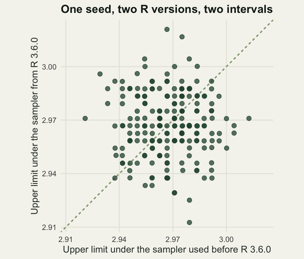
Under the two algorithms the same seed produces different draws immediately: of the first 8 numbers drawn from the 240 quadrats, 0 agree. Across 200 seeds the upper limit of the bootstrap interval differs at 195 of them, by 0.0198 counts per quadrat on average and 0.0667 at the worst seed. What does not change is the distribution. The spread across seeds is 0.0169 under the old sampler and 0.0181 under the new one, and the mean limit is 2.9674 against 2.9675: the two samplers agree about the statistics and disagree about which particular answer this seed gives. That is the honest description of an R upgrade for most analyses: the science survives it and the printed digits do not.
The second omission is below R. The numerical libraries that do matrix arithmetic are chosen at build time, and so is the precision the processor offers for holding a running total. R’s own sum accumulates in a long double, which on an x86 machine is an 80-bit register wider than the doubles being added into it and on Apple Silicon is a plain 64-bit double, because that hardware has no wider format to offer. A matrix product hands the work to whatever BLAS was linked in, which accumulates in its own order and its own width. Those routes are the same sum in arithmetic and can be different sums in floating point, which matters at exactly one place: an equality test.
set.seed(77)
n_try <- 5000
route <- replicate(n_try, {
  z <- rgamma(160, 2, 1)
  w <- z[sample.int(160)]
  long_double <- c(sum(z), sum(w))
  dot_product <- c(as.numeric(rep(1, 160) %*% z), as.numeric(rep(1, 160) %*% w))
  rel <- abs(dot_product[1] - dot_product[2]) / mean(dot_product)
  by_sum <- long_double[1] == long_double[2]
  by_dot <- dot_product[1] == dot_product[2]
  c(equal_long = as.numeric(by_sum),
    equal_dot = as.numeric(by_dot),
    same_verdict = as.numeric(by_sum == by_dot),
    routes_bit_identical = as.numeric(long_double[1] == dot_product[1]),
    digits = if (rel > 0) -log10(rel) else 17)
})
arith <- round(c(trials = n_try,
                 called_equal_by_sum = sum(route["equal_long", ]),
                 called_equal_by_the_dot_product = sum(route["equal_dot", ]),
                 the_two_routes_agreeing_on_the_verdict = sum(route["same_verdict", ]),
                 totals_bit_identical_between_routes = sum(route["routes_bit_identical", ]),
                 called_different_by_the_dot_product_percent =
                   100 * mean(route["equal_dot", ] == 0),
                 median_digits_that_agree = median(route["digits", ]),
                 fewest_digits_that_agree = min(route["digits", ])), 4)
arith
trials
5000.0000
called_equal_by_sum
762.0000
called_equal_by_the_dot_product
762.0000
the_two_routes_agreeing_on_the_verdict
5000.0000
totals_bit_identical_between_routes
5000.0000
called_different_by_the_dot_product_percent
84.7600
median_digits_that_agree
15.4616
fewest_digits_that_agree
14.6881 Each trial takes 160 numbers, reorders them, and adds them up twice by each of two routes. The totals are the same multiset of numbers in a different order, so they are equal in arithmetic, and the only question is whether the machine agrees.
On the build that rendered this page, sum calls the two totals equal in 762 of the 5000 trials and the dot product calls them equal in 762. The two routes reach the same verdict in 5000 trials, and return a total with the same bits in 5000. Read those four counts together, because the pattern in them is the finding. Where sum has a wider register to accumulate in than the doubles going into it, the extra bits absorb the error that reordering introduces: sum then reports equality far more often than the dot product does, the first two counts sit a long way apart, and the last two stay well under the 5000. Where long double is the same 64 bits as a double there is nothing extra to accumulate in, sum behaves the way the dot product does, the first two counts close up on each other, and the last two climb. Same code, same seed, same R version and the same lockfile either way: those counts are a description of the processor.
When the two totals do differ, they differ in the last bits. They still agree to 15.4616 decimal digits at the median trial and never fewer than 14.6881, against the sixteen or so a double carries in total, and the dot product route calls them different in 84.76 per cent of trials. Nothing about that is a bug: it is what floating point addition does, and Goldberg’s survey is the standard place to read why.
It matters because an exact tie is decided by the digits that do not agree. The tie-break in the first half of this post was safe from it, because counts are integers and an integer tie is exact. Change the analysis to rank sites by total cover, or by a weighted mean, or by anything computed through a matrix operation, and a tie between two sites is now settled by the last bits of a sum, which is to say by the BLAS and the accumulator the machine was built with. The lockfile has no field for either.
This section set out to show that a lockfile does not pin the BLAS, and the run has made the point in a stronger form than that. The width of the accumulator is not a library at all. It is a property of the processor, it reaches inside R’s own sum, which no package supplies and no lockfile entry mentions, and there is no version string anywhere in the project folder that records it. Which is why every figure in this section is written into the post as an expression the render evaluates rather than as a digit typed once: the values belong to the machine that built the page, and a number typed by hand here would be a claim about somebody else’s laptop.
The rest of the list is not measurable here and should still be said. The lockfile does not pin the operating system, or the C and Fortran compilers that built the packages from source, or the system libraries that packages such as sf and terra link against, where a GDAL or PROJ upgrade can change a coordinate transformation. It does not pin the data: a lockfile plus a script plus a different extract of the database is a different analysis. And it depends on the archive still being there, so a package pulled from a GitHub branch that its author later deletes is not restorable at any price, which is the strongest practical argument for preferring CRAN sources for anything a result depends on.
Set against that list, what the lockfile does pin, it pins well, and the balance is better than the catalogue of omissions makes it sound. Package behaviour is where the great majority of silent changes live, because packages are where the great majority of the analysis lives: the tie rule, the default link function, the way a smoother chooses its basis dimension, the tolerance at which two coordinates count as the same point. Those are decisions taken by maintainers on their own schedule, and they are the ones a lockfile makes reproducible for the price of one file in the project folder. The R version, the BLAS and the arithmetic of the processor are further down and move much more slowly, and their effects, as measured above, are a change in the last digits and in which particular member of a distribution a seed selects, not a change in what the analysis concludes.
The distinction worth holding on to here separates two things that are usually argued about as one. Reproducing the conclusion is a scientific requirement, and a lockfile helps with it a great deal. Reproducing the exact printed digits is a forensic requirement, useful mainly because it is the only cheap way to show that nothing else has drifted, and for that you need the R version and the system underneath it as well. A reader who reruns your analysis and gets 23.75 per cent where you wrote 23.75 per cent has learned something in five minutes. A reader who gets a figure differing in the second decimal has to work out whether the cause is the sampler, the BLAS or a mistake, and that is the work everybody was trying to avoid.
One omission sits outside the machine altogether and is the largest of the lot. A lockfile records the library, not the sequence of things you typed at the console, so a project can have a perfect lockfile and still produce a figure that no complete run of the script reproduces, because a correction was typed once and never written down. Pinning the environment and running from a clean session are separate habits, and neither substitutes for the other: one fixes what the code is made of, the other fixes what was actually run.
Containers answer most of that list, at a different cost. An image built on a fixed base carries the operating system, the system libraries, the R build and the packages, and it will still run in five years. What you buy that with is a second toolchain to learn, an artefact measured in gigabytes rather than kilobytes, a build recipe that is itself unpinned unless you are careful, and a file that a reader cannot open in a text editor to see what is in it. A lockfile is a few kilobytes of readable text that any R user can act on. For most ecological analyses that is the right trade, and the container is what you reach for when the analysis depends on a compiled geospatial stack or has to survive a decade.
Where to go next
The lockfile is one file in a project layout that has to hold together as a whole, and a reproducible statistical workflow in R sets out the rest of it: where raw data lives, what gets rendered from what, and which files are outputs that should never be edited by hand. Commit the lockfile with the script rather than beside it, which is the habit git for ecologists is about, and the two together answer the question this post opened with, namely which state of the code and the library produced the figure in the manuscript.
Once the environment is pinned, the next thing that goes stale is the intermediate results, and building an analysis pipeline with targets is the tool for that: it records what each result was computed from and rebuilds only what a change invalidates. If the functions you are pinning are your own rather than somebody else’s, put them in a package of your own and version them deliberately, which is where turning your code into an R package starts, and give them the tests from testing your analysis code so that your own tie rules cannot change without something saying so.
References
Sandve GK, Nekrutenko A, Taylor J, Hovig E 2013 PLoS Computational Biology 9(10):e1003285 (10.1371/journal.pcbi.1003285)
Peng RD 2011 Science 334(6060):1226-1227 (10.1126/science.1213847)
Boettiger C 2015 ACM SIGOPS Operating Systems Review 49(1):71-79 (10.1145/2723872.2723882)
Culina A, van den Berg I, Evans S, Sanchez-Tojar A 2020 PLoS Biology 18(7):e3000763 (10.1371/journal.pbio.3000763)
Stodden V, Seiler J, Ma Z 2018 Proceedings of the National Academy of Sciences 115(11):2584-2589 (10.1073/pnas.1708290115)
Goldberg D 1991 ACM Computing Surveys 23(1):5-48 (10.1145/103162.103163)