library(ggplot2)

te_pal <- list(forest = "#275139", green = "#2f8f63", sage = "#93a87f",
               clay = "#b5534e", gold = "#cda23f", line = "#dad9ca",
               ink = "#16241d", paper = "#f5f4ee")

theme_te <- function() {
  theme_minimal(base_size = 12) +
    theme(panel.grid.minor = element_blank(),
          panel.grid.major = element_line(colour = "#e7e6dc"),
          plot.background = element_rect(fill = "#f5f4ee", colour = NA),
          panel.background = element_rect(fill = "#f5f4ee", colour = NA),
          plot.title = element_text(face = "bold", colour = te_pal$ink),
          axis.title = element_text(colour = "#2c3a31"))
}Turning your code into an R package
R
reproducibility
ecology tutorial
ggplot2
Three ecological analyses copied the same R helper and it drifted. Measure what that costs the reported result, then build the minimal package that prevents it.
There are three folders on your laptop. Each one holds an analysis of the same pitfall trap survey: one on grazing, one on elevation, one on the effect of a fire. Each folder holds a file called helpers.R, and each helpers.R holds a function called cpue that turns a site’s trap records into catch per unit effort. The three files began as one file. They were copied, because copying was the fastest way to start the second analysis, and then the third.
Since then the function has been edited four times. Not all four edits went into all three files. Nobody decided that; it is what happens when the same code lives in three places and a person has to remember to visit each of them. The three analyses now compute catch per unit effort in three different ways, and each of them reports a number that goes into a different manuscript.
This post measures that. The survey is simulated, so the answer each analysis should have reported is known throughout, and the drift between the copies can be priced in the units the reader cares about: how far the reported grazing effect, elevation gradient and fire ratio move. Then it builds the thing that makes drift impossible by construction, which is a single source of the function, first as an R/ directory and then as a package. The last measurement is about what a package claims that a sourced file does not: which function a call actually reaches when two of them have the same name.
The sibling post testing your analysis code is the other half of this argument. A package is where shared functions live; a test suite is what makes it safe to change them once three analyses depend on them.
The survey, and the function that summarises it
Eighteen sites, nine of them grazed. Each site is trapped in eight rounds through the season, and every round has its own number of trap nights, because that is how pitfall trapping goes: traps are set when the crew can get to the site and lifted when it can get back. On the ungrazed sites the crew works to the season, so the long rounds fall in the active period. On the grazed sites the protocol is fixed and short, because stock damage the traps if they stay out. A few rounds have no trap nights at all: those traps flooded and the round was lost.
Beetle activity follows the season, falls with elevation, is lower on grazed ground and lower again where the site burned. Some of the specimens cannot be determined to species and are recorded as unidentified, and the proportion that cannot be determined is higher on the grazed sites, where the specimens are damaged.
set.seed(20260816)
n_site  <- 18
n_round <- 8

grazed <- rep(0:1, times = n_site / 2)
elev   <- round(runif(n_site, 380, 1120))
burnt  <- sample(rep(0:1, each = n_site / 2))
u_site <- rnorm(n_site, 0, 0.25)
act    <- c(0.30, 0.55, 0.85, 1.00, 0.95, 0.70, 0.45, 0.25)

rec <- expand.grid(round = seq_len(n_round), site = seq_len(n_site))
rec <- rec[order(rec$site, rec$round), ]
rec$grazed <- grazed[rec$site]
rec$elev   <- elev[rec$site]
rec$burnt  <- burnt[rec$site]

rec$effort <- ifelse(rec$grazed == 1,
                     pmax(2, round(7 + rnorm(nrow(rec), 0, 0.8))),
                     pmax(2, round(2 + 16 * act[rec$round] +
                                     rnorm(nrow(rec), 0, 0.8))))
rec$effort[sample(nrow(rec), round(0.05 * nrow(rec)))] <- 0

lam <- exp(-0.20 + 1.50 * act[rec$round] - 0.45 * rec$grazed -
             0.30 * (rec$elev - 700) / 100 - 0.55 * rec$burnt + u_site[rec$site])
rec$count   <- rpois(nrow(rec), lam * rec$effort)
rec$unident <- rbinom(nrow(rec), rec$count, plogis(-1.7 + 1.1 * rec$grazed +
                                                     0.5 * act[rec$round]))

round(c(sites = n_site, rounds_per_site = n_round, records = nrow(rec),
        specimens = sum(rec$count),
        unidentified = sum(rec$unident),
        rounds_with_no_trap_nights = sum(rec$effort == 0),
        sites_touched_by_a_lost_round = length(unique(rec$site[rec$effort == 0])),
        mean_trap_nights_ungrazed = mean(rec$effort[rec$grazed == 0]),
        mean_trap_nights_grazed = mean(rec$effort[rec$grazed == 1]),
        unidentified_fraction_ungrazed =
          sum(rec$unident[rec$grazed == 0]) / sum(rec$count[rec$grazed == 0]),
        unidentified_fraction_grazed =
          sum(rec$unident[rec$grazed == 1]) / sum(rec$count[rec$grazed == 1])), 4)
sites rounds_per_site
18.0000 8.0000
records specimens
144.0000 2614.0000
unidentified rounds_with_no_trap_nights
635.0000 7.0000
sites_touched_by_a_lost_round mean_trap_nights_ungrazed
4.0000 11.4583
mean_trap_nights_grazed unidentified_fraction_ungrazed
6.5000 0.1988
unidentified_fraction_grazed
0.4362 Two features of that survey are going to matter, and neither is a mistake in the data. Trap nights vary systematically with the season on the ungrazed sites and not on the grazed ones. The unidentified fraction is more than twice as high on the grazed sites as on the ungrazed. Both are ordinary facts about fieldwork, and both mean that a decision inside the summary function has a different effect on one group than on the other. That is the mechanism by which a small coding choice becomes an ecological claim.
Here are the four edits the function has had, in the order they were made.
The first is a bias fix. Catch per unit effort was originally computed as the mean of the per-round rates, mean(count / effort). That gives each round the same weight, including the short ones. The ratio of the sums, sum(count) / sum(effort), weights each round by the effort it actually carried. When effort is correlated with activity, as it is on the ungrazed sites here, the two differ, and the difference is a property of the trapping protocol rather than of the beetles. The person doing the grazing analysis found this and changed her copy.
The second is a crash fix. A round with no trap nights divides by zero. Under the mean of ratios that turns the whole site into a missing value; everybody’s copy broke on the same day, and everybody fixed it.
The third is a determination fix. Unidentified specimens were being counted in the total. The person doing the fire analysis decided they should not be, since a species-level analysis cannot use them, and changed his copy.
The fourth is a unit change. A reviewer asked for rates per 100 trap nights rather than per trap night. Everybody’s numbers changed by a visible factor of one hundred, so everybody made that edit.
make_cpue <- function(e1, e2, e3, e4) {
  function(count, unident, effort) {
    if (e2) {
      k <- effort > 0
      count <- count[k]; unident <- unident[k]; effort <- effort[k]
    }
    if (e3) count <- count - unident
    v <- if (e1) sum(count) / sum(effort) else mean(count / effort)
    if (e4) 100 * v else v
  }
}

site_cpue <- function(fun) sapply(seq_len(n_site), function(s) {
  r <- rec[rec$site == s, ]
  fun(r$count, r$unident, r$effort)
})

cpue_first  <- make_cpue(FALSE, FALSE, FALSE, FALSE)
cpue_shared <- make_cpue(TRUE, TRUE, TRUE, TRUE)
show_site <- function(s) {
  r <- rec[rec$site == s, ]
  cur <- cpue_shared(r$count, r$unident, r$effort)
  c(lost_rounds = sum(r$effort == 0), specimens = sum(r$count),
    unidentified = sum(r$unident), trap_nights = sum(r$effort),
    original_per_trap_night = cpue_first(r$count, r$unident, r$effort),
    current_per_100_trap_nights = cur, current_per_trap_night = cur / 100)
}
print(round(rbind(site_2 = show_site(2), site_9 = show_site(9),
                  site_3 = show_site(3)), 4))
lost_rounds specimens unidentified trap_nights original_per_trap_night
site_2 0 18 11 57 0.3229
site_9 0 45 13 91 0.4264
site_3 1 270 54 81 NaN
current_per_100_trap_nights current_per_trap_night
site_2 12.2807 0.1228
site_9 35.1648 0.3516
site_3 266.6667 2.6667The parameters e1 to e4 stand for the four edits, so that any state of the function can be built and run. A real copy of helpers.R has no such switches: it is one of the sixteen functions this generator can produce, frozen at whichever point its owner stopped editing.
Three sites are enough to see what the edits do. Sites 2 and 9 were trapped in all eight rounds. The original function reports 0.3229 and 0.4264 beetles per trap night for them; the current one reports 12.2807 and 35.1648 per 100 trap nights, which is 0.1228 and 0.3516 in the original’s units. The unit change is the easy part of that gap. The rest is the bias fix and the determination fix working together, and at site 2 they cut the rate by well over half. Site 3 lost a round to flooding, and the original function returns NaN for it, because one of the eight per-round rates it averages is a count divided by zero trap nights. That is the crash everybody fixed on the same day, and it is the only one of the four edits the code itself insisted on.
Three analyses, three copies, three answers
The grazing analysis reports the percentage difference in catch per unit effort between grazed and ungrazed sites. The elevation analysis reports the slope of catch per unit effort against elevation, per 100 metres. The fire analysis reports the ratio of burnt to unburnt. None of these three quantities is exotic; each is the sentence in the abstract.
Each analysis runs against the copy of cpue that is in its own folder. The grazing folder has the bias fix, the crash fix and the unit change. The elevation folder has the crash fix and the unit change and nothing else. The fire folder has the crash fix, the determination fix and the unit change. The shared source, the state the function is in today if you look at the most recently edited copy of each edit, has all four.
ana_graze <- function(v) 100 * (mean(v[grazed == 1]) - mean(v[grazed == 0])) /
  mean(v[grazed == 0])
ana_elev  <- function(v) unname(coef(lm(v ~ I(elev / 100)))[2])
ana_fire  <- function(v) mean(v[burnt == 1]) / mean(v[burnt == 0])

copy_flags <- data.frame(
  copy = c("Grazing", "Elevation", "Fire", "Shared source"),
  e1 = c(TRUE, FALSE, FALSE, TRUE), e2 = c(TRUE, TRUE, TRUE, TRUE),
  e3 = c(FALSE, FALSE, TRUE, TRUE), e4 = c(TRUE, TRUE, TRUE, TRUE),
  stringsAsFactors = FALSE)
print(copy_flags)
copy e1 e2 e3 e4
1 Grazing TRUE TRUE FALSE TRUE
2 Elevation FALSE TRUE FALSE TRUE
3 Fire FALSE TRUE TRUE TRUE
4 Shared source TRUE TRUE TRUE TRUEcpue_of <- function(i) make_cpue(copy_flags$e1[i], copy_flags$e2[i],
copy_flags$e3[i], copy_flags$e4[i])
v_shared <- site_cpue(cpue_of(4))
reported <- c(graze = ana_graze(site_cpue(cpue_of(1))),
elev = ana_elev(site_cpue(cpue_of(2))),
fire = ana_fire(site_cpue(cpue_of(3))))
correct <- c(graze = ana_graze(v_shared), elev = ana_elev(v_shared),
fire = ana_fire(v_shared))
shift <- 100 * (abs(reported) - abs(correct)) / abs(correct)
round(c(grazing_reported_percent_difference = reported["graze"],
grazing_with_the_shared_source = correct["graze"],
elevation_reported_slope_per_100m = reported["elev"],
elevation_with_the_shared_source = correct["elev"],
fire_reported_ratio = reported["fire"],
fire_with_the_shared_source = correct["fire"]), 4)grazing_reported_percent_difference.graze
-61.3394
grazing_with_the_shared_source.graze
-72.7307
elevation_reported_slope_per_100m.elev
-42.8106
elevation_with_the_shared_source.elev
-36.6740
fire_reported_ratio.fire
0.5509
fire_with_the_shared_source.fire
0.5443 round(c(grazing_shift_percent = shift["graze"],
elevation_shift_percent = shift["elev"],
fire_shift_percent = shift["fire"],
analyses_that_disagree_with_the_shared_source = sum(abs(shift) > 1e-8),
analyses_still_carrying_the_bias = sum(!copy_flags$e1[1:3]),
edits_in_every_copy = sum(apply(copy_flags[1:3, 2:5], 2, all)),
edits_in_only_one_copy = sum(colSums(copy_flags[1:3, 2:5]) == 1)), 4) grazing_shift_percent.graze
-15.6623
elevation_shift_percent.elev
16.7328
fire_shift_percent.fire
1.2166
analyses_that_disagree_with_the_shared_source
3.0000
analyses_still_carrying_the_bias
2.0000
edits_in_every_copy
2.0000
edits_in_only_one_copy
2.0000 edit_lab <- c("1. Bias fix\n(ratio of sums)", "2. Crash fix\n(drop lost rounds)",
"3. Determination fix\n(drop unidentified)",
"4. Unit change\n(per 100 trap nights)")
grid_df <- data.frame(
copy = factor(rep(copy_flags$copy, each = 4), levels = copy_flags$copy),
edit = factor(rep(edit_lab, times = 4), levels = rev(edit_lab)),
present = as.vector(t(as.matrix(copy_flags[, 2:5]))))
grid_df$state <- factor(ifelse(grid_df$present, "in this copy", "missing"),
levels = c("in this copy", "missing"))
ggplot(grid_df, aes(copy, edit, fill = state)) +
geom_tile(colour = te_pal$ink, linewidth = 0.6, width = 0.92, height = 0.92) +
scale_fill_manual(values = c(te_pal$forest, te_pal$paper), name = NULL) +
labs(x = NULL, y = NULL,
title = "The two edits nobody could miss reached every copy") +
theme_te() +
theme(legend.position = "top",
panel.grid.major = element_blank(),
axis.text.y = element_text(size = 8.5, colour = te_pal$ink),
axis.text.x = element_text(size = 9.5, colour = te_pal$ink))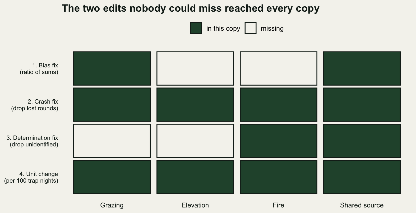
All three analyses disagree with the shared source, and two of the three still carry the bias the first edit was made to remove. The sizes of the disagreement are worth looking at one at a time.
The grazing analysis reports that grazed sites hold 61.3394 per cent fewer beetles per trap night than ungrazed sites. With the shared source it is 72.7307 per cent, so the reported effect is understated by 15.6623 per cent of the shared source’s value. The cause is the missing determination fix: unidentified specimens are still in the total, and because more than twice as many specimens go undetermined on grazed ground, leaving them in props up the grazed sites and flattens the contrast.
The elevation analysis reports a slope of 42.8106 fewer beetles per 100 trap nights per 100 metres of elevation, where the shared source gives 36.674: the gradient is overstated by 16.7328 per cent. Two edits are missing from that copy and they pull against each other. Leaving unidentified specimens in the total adds most to the sites that caught most, which are the low ones, and on its own steepens the slope to 48.4878. The unweighted mean of per-round rates adds most where effort varied most, and on its own flattens it to 32.7227. What lands in the manuscript is 42.8106, so the two partly cancel, and neither is visible in the output.
The fire analysis reports a burnt to unburnt ratio of 0.5509 against the shared source’s 0.5443, a difference of 1.2166 per cent. That is the awkward one. It is far too small to notice, far too small to change any conclusion in the paper, and it is not zero. There is no threshold below which a number that came out of the wrong version of a function becomes the number you meant to report.
Nothing in any of the three runs produced a warning, an error or a missing value. Each folder contains a script that runs cleanly and a function that is a defensible way of computing catch per unit effort. The problem is not in any one folder. It is that there are three of them.
The pattern in the tile grid is not random, and it is the reason this failure is so durable. Two of the four edits reached every copy and two reached exactly one. The two that travelled are the two that announced themselves. The crash fix travelled because the code stopped working: a missing value is a message from the machine, addressed to the person, saying that something must change. The unit change travelled because a reviewer asked for it in writing and because everybody’s numbers moved by a factor of one hundred, which nobody can look at and not notice.
The two that stayed put moved the reported answers by as much as 16.7328 per cent and changed nothing else. There was no message and no reviewer, only a person who thought about the problem and improved her own copy. The edits that most need to propagate are exactly the ones with no mechanism to make them propagate, and that asymmetry is a property of the arrangement rather than of the people. It cannot be fixed by being more careful, because being careful is what produced the edit in the first place.
Sixteen versions of one function
Four edits give sixteen possible states of cpue, and every one of them is a file somebody could have on their laptop right now. Running all sixteen against all three analyses turns the vague worry into a distribution.
combos <- expand.grid(e1 = c(FALSE, TRUE), e2 = c(FALSE, TRUE),
                      e3 = c(FALSE, TRUE), e4 = c(FALSE, TRUE))
res <- t(sapply(seq_len(nrow(combos)), function(i) {
  v <- site_cpue(make_cpue(combos$e1[i], combos$e2[i], combos$e3[i],
                           combos$e4[i]))
  if (!all(is.finite(v))) return(c(NA_real_, NA_real_, NA_real_))
  c(ana_graze(v), ana_elev(v), ana_fire(v))
}))
colnames(res) <- c("graze", "elev", "fire")
full <- which(combos$e1 & combos$e2 & combos$e3 & combos$e4)
err  <- 100 * (abs(res) - rep(abs(res[full, ]), each = nrow(res))) /
  rep(abs(res[full, ]), each = nrow(res))
runs <- is.finite(res[, "graze"])
print(cbind(combos, round(res, 4)))
e1 e2 e3 e4 graze elev fire
1 FALSE FALSE FALSE FALSE NA NA NA
2 TRUE FALSE FALSE FALSE -61.3394 -0.4849 0.5754
3 FALSE TRUE FALSE FALSE -55.8946 -0.4281 0.5826
4 TRUE TRUE FALSE FALSE -61.3394 -0.4849 0.5754
5 FALSE FALSE TRUE FALSE NA NA NA
6 TRUE FALSE TRUE FALSE -72.7307 -0.3667 0.5443
7 FALSE TRUE TRUE FALSE -69.1007 -0.3272 0.5509
8 TRUE TRUE TRUE FALSE -72.7307 -0.3667 0.5443
9 FALSE FALSE FALSE TRUE NA NA NA
10 TRUE FALSE FALSE TRUE -61.3394 -48.4878 0.5754
11 FALSE TRUE FALSE TRUE -55.8946 -42.8106 0.5826
12 TRUE TRUE FALSE TRUE -61.3394 -48.4878 0.5754
13 FALSE FALSE TRUE TRUE NA NA NA
14 TRUE FALSE TRUE TRUE -72.7307 -36.6740 0.5443
15 FALSE TRUE TRUE TRUE -69.1007 -32.7227 0.5509
16 TRUE TRUE TRUE TRUE -72.7307 -36.6740 0.5443distinct <- apply(round(res[runs, ], 8), 2, function(z) length(unique(z)))
round(c(possible_versions = nrow(combos),
versions_that_return_a_missing_value = sum(!runs),
versions_that_run = sum(runs),
distinct_grazing_answers = distinct["graze"],
distinct_elevation_answers = distinct["elev"],
distinct_fire_answers = distinct["fire"],
worst_grazing_error_percent = max(abs(err[runs, "graze"])),
worst_elevation_error_percent = max(abs(err[runs, "elev"])),
worst_fire_error_percent = max(abs(err[runs, "fire"])),
versions_that_get_grazing_right = sum(abs(err[runs, "graze"]) < 1e-8)), 4) possible_versions versions_that_return_a_missing_value
16.0000 4.0000
versions_that_run distinct_grazing_answers.graze
12.0000 4.0000
distinct_elevation_answers.elev distinct_fire_answers.fire
8.0000 4.0000
worst_grazing_error_percent worst_elevation_error_percent
23.1485 99.1077
worst_fire_error_percent versions_that_get_grazing_right
7.0489 4.0000 ana_lab <- c(graze = "Grazing effect", elev = "Elevation slope",
fire = "Fire ratio")
role_lab <- c("One of the twelve runnable versions",
"The version this analysis uses")
spread_df <- data.frame(
value = as.vector(err[runs, ]),
analysis = factor(rep(ana_lab, each = sum(runs)), levels = rev(ana_lab)),
role = factor(role_lab[1], levels = role_lab))
# stack points that are within one marker of each other on the drawn axis, not
# only points that are exactly equal: the axis spans 144 per cent across the
# panel, so a marker is about 2 per cent wide. Grouping on the gap rather than
# on a rounded value means no cluster gets split by a bin edge.
spread_bin <- ave(spread_df$value, spread_df$analysis, FUN = function(z) {
o <- order(z)
g <- numeric(length(z))
g[o] <- cumsum(c(0, diff(z[o]) > 2))
g
})
# centre each stack on its own row by removing the mean offset, so a tall column
# straddles the row line instead of climbing towards the row above it.
spread_df$y <- as.numeric(spread_df$analysis) +
ave(spread_df$value, spread_df$analysis, spread_bin,
FUN = function(z) {
o <- 0.13 * (rank(z, ties.method = "first") - 1)
o - mean(o)
})
mine_df <- data.frame(value = as.numeric(shift),
analysis = factor(ana_lab, levels = rev(ana_lab)),
role = factor(role_lab[2], levels = role_lab))
mine_df$y <- as.numeric(mine_df$analysis)
ggplot(rbind(spread_df, mine_df), aes(value, y, colour = role, shape = role,
size = role)) +
geom_vline(xintercept = 0, colour = te_pal$sage, linetype = 2, linewidth = 0.8) +
geom_point(stroke = 1.4, alpha = 0.9) +
annotate("text", x = 1.5, y = 3.72, label = "the shared source", hjust = 0,
size = 3.2, colour = "#2c3a31") +
scale_colour_manual(values = c(te_pal$forest, te_pal$clay), name = NULL) +
scale_shape_manual(values = c(16, 1), name = NULL) +
scale_size_manual(values = c(3, 6.5), name = NULL) +
scale_y_continuous(breaks = seq_along(ana_lab), labels = rev(ana_lab),
limits = c(0.6, 3.85)) +
scale_x_continuous(limits = c(-104, 40)) +
labs(x = "Difference from the shared source (per cent of the shared answer)",
y = NULL,
title = "Twelve runnable copies of one helper, and they do not agree") +
theme_te() +
theme(legend.position = "top",
axis.text.y = element_text(colour = te_pal$ink))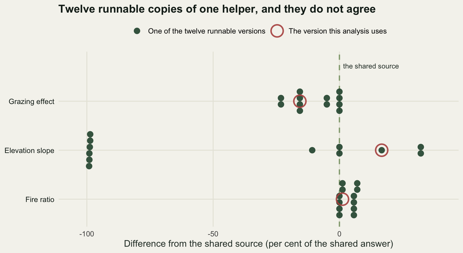
Four of the sixteen return a missing value for at least one site, and they are the four that have neither the bias fix nor the crash fix. That is the good case: the script stops being able to produce a figure and somebody investigates within the hour. The remaining 12 all run. They give 4 different answers to the grazing question, 8 to the elevation question and 4 to the fire question.
The count of distinct answers is smaller than 12 in every case, and the reason is worth a moment. Which edits change your number depends on what you report. The crash fix never separates two runnable versions at all, because a ratio of sums handles a zero-effort round without being told to, so among versions that run it only ever matters in company with the bias fix, which has already dealt with the problem. The grazing analysis reports a ratio between two groups of sites, so the unit change cancels out of it as well. That leaves the bias fix and the determination fix, two choices with two states each: 4 outcomes from 12 files, and 4 of the 12 give the grazing answer the shared source gives. The elevation analysis reports a slope in the helper’s own units, so the unit change does not cancel, and 8 distinct answers come out of the same 12 files. The fire analysis is a ratio again, and lands back at 4.
None of this is knowable from the function. You cannot look at cpue and say which of its edits your analysis is sensitive to; that depends on the quantity at the far end of the script, three steps later. Which is a long way of saying that the only safe assumption is that every edit matters to every analysis, and the only arrangement that makes that assumption cheap is one copy of the code.
The elevation row of the figure is the one to look at last. Half of its versions sit at about minus 99 per cent, which is not a subtle bias: it is the factor of one hundred from the missing unit change, showing up as a slope a hundred times shallower. That kind of divergence is safe, in the sense that anybody who reads the number will see it. The dangerous versions are the ones that miss the shared answer by tens of per cent rather than by a factor of a hundred, which is close enough to the right order to pass into a manuscript unquestioned.
How often does a copy fall behind?
The three folders in this post were assigned their edits by hand, to tell a story. The general question is what happens on average, and that can be answered exactly rather than by simulation.
Take a project with n copies of the helper, over which k edits are made. Each edit is made in whichever copy the person happened to be working in, and then copied into each other copy with probability p. Write p as diligence: p equal to one is a person who never forgets, p equal to a half is a person who copies the change over about half the time.
For a single edit to reach all n copies, all n - 1 non-authors have to receive it, which happens with probability p to the power n - 1, whoever wrote it. Edits are independent, so all k edits are everywhere with probability p to the power k times n - 1. For one particular copy, an edit is present if that copy authored it, with probability one over n, or if it was copied in, so the chance any given edit is in any given copy is one over n plus the rest of the mass times p.
k_edit <- 4
p_all  <- function(n, p, k = k_edit) p^(k * (n - 1))
q_one  <- function(n, p) 1 / n + (1 - 1 / n) * p
p_for  <- function(n, target = 0.95, k = k_edit) target^(1 / (k * (n - 1)))

round(c(edits = k_edit, copies = 3,
        all_current_at_diligence_half = 100 * p_all(3, 0.5),
        all_current_at_diligence_three_quarters = 100 * p_all(3, 0.75),
        all_current_at_diligence_nine_tenths = 100 * p_all(3, 0.9),
        stale_somewhere_at_nine_tenths = 100 * (1 - p_all(3, 0.9)),
        diligence_needed_for_95_percent_two_copies = 100 * p_for(2),
        diligence_needed_for_95_percent_three_copies = 100 * p_for(3),
        diligence_needed_for_95_percent_five_copies = 100 * p_for(5)), 4)
edits
4.0000
copies
3.0000
all_current_at_diligence_half
0.3906
all_current_at_diligence_three_quarters
10.0113
all_current_at_diligence_nine_tenths
43.0467
stale_somewhere_at_nine_tenths
56.9533
diligence_needed_for_95_percent_two_copies
98.7259
diligence_needed_for_95_percent_three_copies
99.3609
diligence_needed_for_95_percent_five_copies
99.6799 wt <- apply(combos, 1, function(r) prod(ifelse(r, q_one(3, 0.5),
1 - q_one(3, 0.5))))
wrun <- wt * runs
round(c(chance_a_copy_has_every_edit_percent = 100 * wt[full],
chance_a_copy_returns_a_missing_value_percent = 100 * sum(wt[!runs]),
chance_a_copy_runs_and_is_wrong_percent = 100 * (sum(wrun) - wt[full]),
expected_grazing_error_percent =
sum(wrun * abs(err[, "graze"]), na.rm = TRUE) / sum(wrun),
expected_elevation_error_percent =
sum(wrun * abs(err[, "elev"]), na.rm = TRUE) / sum(wrun),
expected_fire_error_percent =
sum(wrun * abs(err[, "fire"]), na.rm = TRUE) / sum(wrun),
copies_a_single_edit_reaches_by_hand = 1 + 2 * 0.5,
copies_a_single_edit_reaches_from_one_source = 3), 4) chance_a_copy_has_every_edit_percent
19.7531
chance_a_copy_returns_a_missing_value_percent
11.1111
chance_a_copy_runs_and_is_wrong_percent
69.1358
expected_grazing_error_percent
6.6765
expected_elevation_error_percent
40.4701
expected_fire_error_percent
2.2213
copies_a_single_edit_reaches_by_hand
2.0000
copies_a_single_edit_reaches_from_one_source
3.0000 pg <- seq(0.5, 1, length.out = 401)
dil_df <- do.call(rbind, lapply(c(2, 3, 5), function(n)
data.frame(p = 100 * pg, stale = 100 * (1 - p_all(n, pg)),
copies = factor(paste(n, "copies"),
levels = c("2 copies", "3 copies", "5 copies")))))
ggplot(dil_df, aes(p, stale, colour = copies)) +
geom_hline(yintercept = 5, linetype = 2, colour = te_pal$clay, linewidth = 0.8) +
annotate("text", x = 50.5, y = 10.5, label = "a one in twenty risk", hjust = 0,
size = 3.2, colour = te_pal$clay) +
geom_line(linewidth = 1.2) +
scale_colour_manual(values = c(te_pal$sage, te_pal$green, te_pal$forest),
name = NULL) +
scale_y_continuous(limits = c(0, 100)) +
labs(x = "Chance an edit gets copied into another file (per cent)",
y = "Chance at least one copy is stale (per cent)",
title = "Three copies: copying nine edits in ten leaves one stale more often than not") +
theme_te() +
theme(legend.position = "top")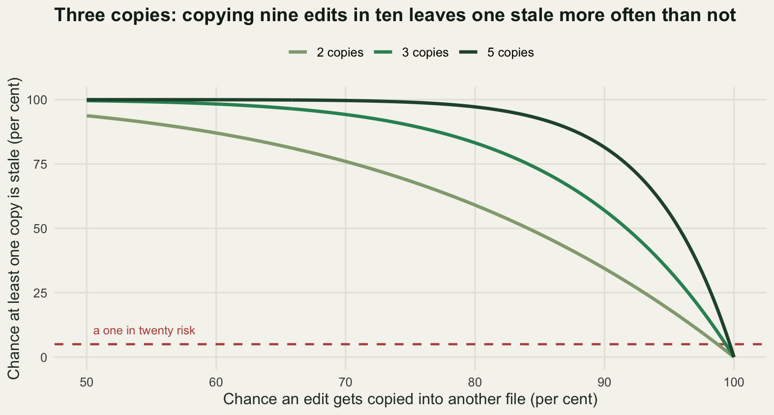
The numbers are not close. With three copies and four edits, a person who copies every change into every other file nine times out of ten ends the project with a stale copy somewhere 56.9533 per cent of the time. To get that risk down to one in twenty you would have to be right 99.3609 per cent of the time, and with five copies, 99.6799 per cent. Human diligence is not the failure here; the arithmetic is simply not survivable. Every extra copy multiplies the number of chances to forget.
At a diligence of one half, a given copy holds every edit 19.7531 per cent of the time, returns a missing value 11.1111 per cent of the time, and runs while being wrong the remaining 69.1358 per cent. Averaged over the copies that run at all, the grazing answer is out by 6.6765 per cent and the fire answer by 2.2213 per cent. The elevation figure is dominated by the factor of one hundred, so its average of 40.4701 per cent is really two populations and not a typical error at all.
The model behind those numbers is deliberately generous. It assumes edits are independent, that nobody ever copies a stale version over a current one, and that the person copying does not make a mistake while doing it. All three assumptions favour copying. It also assumes the copies are only ever edited by the people in this project, which stops being true the moment somebody sends the folder to a collaborator. What the model does capture is the only structural fact that matters here: the number of things that have to go right grows with the number of copies times the number of edits, and each of them is a separate act of memory.
One source: from an R directory to a package
The fix is not more diligence. It is to have one copy of the function, so that the question of which folder holds which version cannot be asked. The smallest version of that is a directory of function files that every analysis reads at the top:
# analysis.R, in each project folder
source("../shared/R/cpue.R")
That single line removes the whole of the last three sections. There is one definition; an edit reaches every analysis the next time it runs; the tile grid becomes one column. It is a real improvement and for a two-person, two-analysis project it may be all you need.
What it does not give you is anything that a stranger, or you in eighteen months, can rely on. The relative path breaks the moment a folder moves. There is no version, so a manuscript cannot say which state of the function produced its numbers. There is nothing that records that cpue needs the stats package. Nothing runs the tests. And, the subject of the next section, source drops the function into your global environment, where it silently outranks everything with the same name.
A package answers all five. It is a directory with a fixed shape, and the shape is the whole of the specification:
# beetletools/
#   DESCRIPTION        name, version, what it needs to run
#   NAMESPACE          what it makes public, what it takes from elsewhere
#   R/cpue.R           the function definitions
#   man/cpue.Rd        the help page, so that ?cpue works
#   tests/testthat/    the checks that R CMD check will run for you
DESCRIPTION is the part that turns a folder into a thing with an identity. Five fields is enough:
# beetletools/DESCRIPTION
Package: beetletools
Version: 0.4.0
Title: Summaries for the upland pitfall trap survey
Depends: R (>= 4.1)
Imports: stats
NAMESPACE is a short file with a large meaning, and it is the subject of the next section:
# beetletools/NAMESPACE
export(cpue)
importFrom(stats, sd)
Then the function itself goes in R/cpue.R. It is the same function, with a block of comment lines above it that carry the documentation. Writing those comments is the one piece of real work in the move, and it is work worth doing for its own sake, because it forces you to say in a sentence what the function returns and in what units, which is the question every one of the four edits was about:
# beetletools/R/cpue.R
#' Catch per unit effort for one site
#'
#' @param count Specimens caught in each trapping round.
#' @param unident Of those, the ones not determined to species.
#' @param effort Trap nights in each round. Rounds with zero are dropped.
#' @return Determined specimens per 100 trap nights, as one number.
#' @export
cpue <- function(count, unident, effort) {
  stopifnot(length(count) == length(effort), length(unident) == length(effort))
  keep <- effort > 0
  100 * sum(count[keep] - unident[keep]) / sum(effort[keep])
}
The tests you already wrote go under tests/. From a session with the package directory open, three calls do the rest. They are not run here because this post has to render with nothing installed beyond ggplot2:
# in the beetletools directory, using the devtools package
devtools::document()   # writes man/ and NAMESPACE from the roxygen comments
devtools::check()      # R CMD check: does it install, do the examples run, do the tests pass
devtools::install()    # put it in the library, so library(beetletools) works anywhere
What usethis, devtools and roxygen2 add is typing speed and nothing else. usethis::create_package() writes the DESCRIPTION you saw above. roxygen2 turns comments above the function into the .Rd file and the NAMESPACE entries, so that the documentation lives next to the code it documents. devtools::check() runs R CMD check, which is a program that ships with R. Every one of those files can be written by hand in a text editor, and writing the first one by hand is the fastest way to stop treating a package as a ceremony.
The thing that changes on the day the package exists is not the code. It is that library(beetletools) means the same thing in every folder, on every machine, and the version number in DESCRIPTION is something a manuscript can cite. The tile grid in the first figure can no longer have more than one column.
That cuts both ways, and the honest version of the argument has to say so. With three hand-kept copies and a diligence of one half, a single edit reaches 2 of the 3 copies on average. From one source it reaches 3 of 3, immediately, whether it was a fix or a mistake. Shared code raises the cost of a bad change in exactly the proportion that it lowers the cost of a good one, which is why testing your analysis code is the companion to this post and not an optional extra.
NAMESPACE is a claim about which function you get
Here is a habit almost every ecologist has picked up: a helper that rescales a covariate so that the largest value is one, written into helpers.R and given the obvious name.
# helpers.R, the version that causes the trouble
scale <- function(x) x / max(abs(x))
scale is a base R function. It centres and standardises, and the standardised coefficients that come out of a model fitted to scaled covariates are what people use to say which driver matters most. When the helper file is sourced, its scale goes into the global environment, and the global environment is searched before every attached package, including base. From then on the same call means something different.
A second study makes the point: 40 sites, catch per unit effort computed with the shared helper, and three measured drivers. The analysis standardises all three and compares the size of the fitted coefficients.
set.seed(4162)
n2      <- 40
elev2   <- round(runif(n2, 380, 1120))
ph2     <- round(rnorm(n2, 6.20, 0.42), 2)
litter2 <- round(pmax(0.5, rnorm(n2, 3.0, 1.6)), 1)

rec2 <- expand.grid(round = 1:6, site = seq_len(n2))
rec2$effort  <- pmax(2, round(rnorm(nrow(rec2), 9, 2.4)))
rate2 <- exp(0.30 - 0.34 * (elev2[rec2$site] - 700) / 100 +
               0.55 * (ph2[rec2$site] - 6.2) + 0.11 * (litter2[rec2$site] - 3.0))
rec2$count   <- rpois(nrow(rec2), rate2 * rec2$effort)
rec2$unident <- rbinom(nrow(rec2), rec2$count, 0.12)
cpue2 <- sapply(seq_len(n2), function(s) {
  r <- rec2[rec2$site == s, ]
  cpue_shared(r$count, r$unident, r$effort)
})

field_scale <- function(x) x / max(abs(x))
round(c(sites = n2, records = nrow(rec2),
        median_cpue_per_100_trap_nights = median(cpue2),
        elevation_sd = sd(elev2), elevation_max = max(elev2),
        soil_ph_sd = sd(ph2), soil_ph_max = max(ph2),
        litter_sd = sd(litter2), litter_max = max(litter2),
        elevation_max_over_sd = max(abs(elev2)) / sd(elev2),
        soil_ph_max_over_sd = max(abs(ph2)) / sd(ph2),
        litter_max_over_sd = max(abs(litter2)) / sd(litter2)), 4)
sites records
40.0000 240.0000
median_cpue_per_100_trap_nights elevation_sd
111.9318 234.9315
elevation_max soil_ph_sd
1117.0000 0.4441
soil_ph_max litter_sd
7.2200 1.5263
litter_max elevation_max_over_sd
7.2000 4.7546
soil_ph_max_over_sd litter_max_over_sd
16.2569 4.7172 The ratio of the largest value to the standard deviation is the whole story in advance. Elevation’s maximum sits under five standard deviations from zero; soil pH’s sits above sixteen, because pH is a number near seven whose interesting variation is a few tenths. Dividing by the maximum leaves pH almost constant, and a coefficient on an almost constant predictor has to be large to do the same work.
Now the same analysis function, run in two environments. In the first, scale resolves to base R’s. In the second, the helper’s definition sits in between, exactly as a sourced file would.
rank_drivers <- function() {
  z_elev   <- as.numeric(scale(elev2))
  z_ph     <- as.numeric(scale(ph2))
  z_litter <- as.numeric(scale(litter2))
  fit <- lm(cpue2 ~ z_elev + z_ph + z_litter)
  list(coef = coef(fit)[-1], r2 = summary(fit)$r.squared,
       fitted = unname(fitted(fit)))
}

env_clean  <- new.env(parent = globalenv())
env_masked <- new.env(parent = globalenv())
assign("scale", field_scale, envir = env_masked)

as_pkg  <- rank_drivers; environment(as_pkg)  <- env_clean
sourced <- rank_drivers; environment(sourced) <- env_masked
fit_pkg <- as_pkg()
fit_src <- sourced()

print(round(rbind(base_scale = fit_pkg$coef, helper_scale = fit_src$coef), 4))
z_elev z_ph z_litter
base_scale -105.337 39.6007 30.1159
helper_scale -500.833 643.7841 142.0618rank_pkg <- names(sort(-abs(fit_pkg$coef)))
rank_src <- names(sort(-abs(fit_src$coef)))
print(rbind(base_scale = rank_pkg, helper_scale = rank_src)) [,1] [,2] [,3]
base_scale "z_elev" "z_ph" "z_litter"
helper_scale "z_ph" "z_elev" "z_litter"pair_flip <- function(a, b) {
ij <- which(upper.tri(matrix(0, length(a), length(a))), arr.ind = TRUE)
sum(sign(abs(a[ij[, 1]]) - abs(a[ij[, 2]])) *
sign(abs(b[ij[, 1]]) - abs(b[ij[, 2]])) < 0)
}
round(c(r_squared_base = fit_pkg$r2, r_squared_helper = fit_src$r2,
largest_fitted_value_difference = max(abs(fit_pkg$fitted -
fit_src$fitted)),
driver_pairs = choose(3, 2),
driver_pairs_reordered = pair_flip(fit_pkg$coef, fit_src$coef),
elevation_coefficient_inflated = abs(fit_src$coef[1] / fit_pkg$coef[1]),
soil_ph_coefficient_inflated = abs(fit_src$coef[2] / fit_pkg$coef[2]),
litter_coefficient_inflated = abs(fit_src$coef[3] / fit_pkg$coef[3])), 4) r_squared_base r_squared_helper
0.8604 0.8604
largest_fitted_value_difference driver_pairs
0.0000 3.0000
driver_pairs_reordered elevation_coefficient_inflated.z_elev
1.0000 4.7546
soil_ph_coefficient_inflated.z_ph litter_coefficient_inflated.z_litter
16.2569 4.7172 The model is the same model. Both fits report an R squared of 0.8604, and the largest difference between the two sets of fitted values is 0 at the four decimals printed, because rescaling a predictor by a constant cannot change a linear fit. What changes is the size of the coefficients, each one inflated by exactly that predictor’s maximum divided by its standard deviation: 4.7546 for elevation, 16.2569 for soil pH, 4.7172 for litter depth. Since those factors differ, the ordering changes. With base R’s scale the strongest driver is elevation, at 105.337 against soil pH’s 39.6007. With the helper’s scale the strongest driver is soil pH, at 643.7841 against elevation’s 500.833. One of the 3 pairwise orderings reverses, and it is the pair the paper is about.
Nothing warns you. There is no message, the model summary looks the way a model summary looks, and the sentence that comes out of it changes from “elevation is the dominant driver” to “soil pH is the dominant driver”. A reader of the script sees scale(ph2) and reads it as the base R function, because that is what it says.
The call scale(ph2) is identical in both runs. What differs is which definition it reaches, and that is settled entirely by the environment the calling function was defined in.
R settles that by walking a chain of environments and taking the first scale it finds. Four chains are worth building, because they are the four situations you will actually be in. Nothing masked. A helper file sourced into the session. The analyst’s own redefinition sitting in the global environment. And a function living inside a package, whose chain runs through the package’s own namespace and then base before it ever reaches the session.
env_user <- new.env(parent = globalenv())          # the analyst redefines the name
assign("scale", function(x) x - mean(x), envir = env_user)
env_srcd <- new.env(parent = env_user)             # a sourced helper, ahead of base
assign("scale", field_scale, envir = env_srcd)
base_link <- new.env(parent = env_user)            # base, ahead of the session
assign("scale", get("scale", envir = baseenv()), envir = base_link)
env_pkgns <- new.env(parent = base_link)           # a function inside a package

first_z <- function() as.numeric(scale(ph2))[1]
reach <- sapply(list(nothing_masked = env_clean, sourced_helper = env_srcd,
                     user_redefinition = env_user, inside_a_package = env_pkgns),
                function(e) { f <- first_z; environment(f) <- e; f() })
explicit <- get("scale", envir = baseenv())
round(c(soil_ph_at_site_1 = ph2[1], mean_soil_ph = mean(ph2),
        sd_soil_ph = sd(ph2), max_soil_ph = max(ph2),
        value_with_nothing_masked = reach["nothing_masked"],
        value_with_the_sourced_helper = reach["sourced_helper"],
        value_with_a_user_redefinition = reach["user_redefinition"],
        value_inside_a_package = reach["inside_a_package"],
        value_from_an_explicit_base_lookup = as.numeric(explicit(ph2))[1]), 4)
soil_ph_at_site_1
6.0100
mean_soil_ph
6.2488
sd_soil_ph
0.4441
max_soil_ph
7.2200
value_with_nothing_masked.nothing_masked
-0.5376
value_with_the_sourced_helper.sourced_helper
0.8324
value_with_a_user_redefinition.user_redefinition
-0.2388
value_inside_a_package.inside_a_package
-0.5376
value_from_an_explicit_base_lookup
-0.5376 One call, four chains, and three different answers: -0.5376, 0.8324, -0.2388, and then -0.5376 again. The last one is what a package buys you. The function inside the package reaches base R’s scale even though the session it is running in has redefined the name, because its chain puts the package’s own namespace and then base ahead of the global environment. The same protection is available to a sourced helper only by asking for the definition explicitly, which is what base::scale does: it returns -0.5376 regardless of what anybody has defined anywhere.
That is what the export line in NAMESPACE is for. A package states which of its functions are public, so that everything else it defines stays private and cannot collide with anything. When you attach it, R prints a message naming every object it masks, so a collision with base R is announced at the moment it happens rather than discovered in a coefficient six months later. A sourced file gets none of that. It is dropped into the global environment, which sits ahead of every package on the search path, it makes every function in the file public whether you meant it or not, and R says nothing at all.
drv_lab <- c("Elevation", "Soil pH", "Litter depth")
panel_lab <- c("Standardised with base R scale()",
               "Standardised with the helper's scale()")
mask_df <- data.frame(
  driver = factor(rep(drv_lab, 2), levels = drv_lab),
  value = abs(c(fit_pkg$coef, fit_src$coef)),
  panel = factor(rep(panel_lab, each = 3), levels = panel_lab))

ggplot(mask_df, aes(driver, value, fill = driver)) +
  geom_col(width = 0.62, show.legend = FALSE) +
  geom_text(aes(label = sprintf("%.2f", value)), vjust = -0.4, size = 3.4,
            colour = te_pal$ink) +
  facet_wrap(~panel, scales = "free_y") +
  scale_fill_manual(values = c(te_pal$forest, te_pal$gold, te_pal$sage)) +
  scale_y_continuous(expand = expansion(mult = c(0, 0.18))) +
  labs(x = NULL, y = "Absolute standardised coefficient",
       title = "One masked function name, a different most important driver") +
  theme_te() +
  theme(strip.text = element_text(colour = te_pal$ink, face = "bold", size = 9))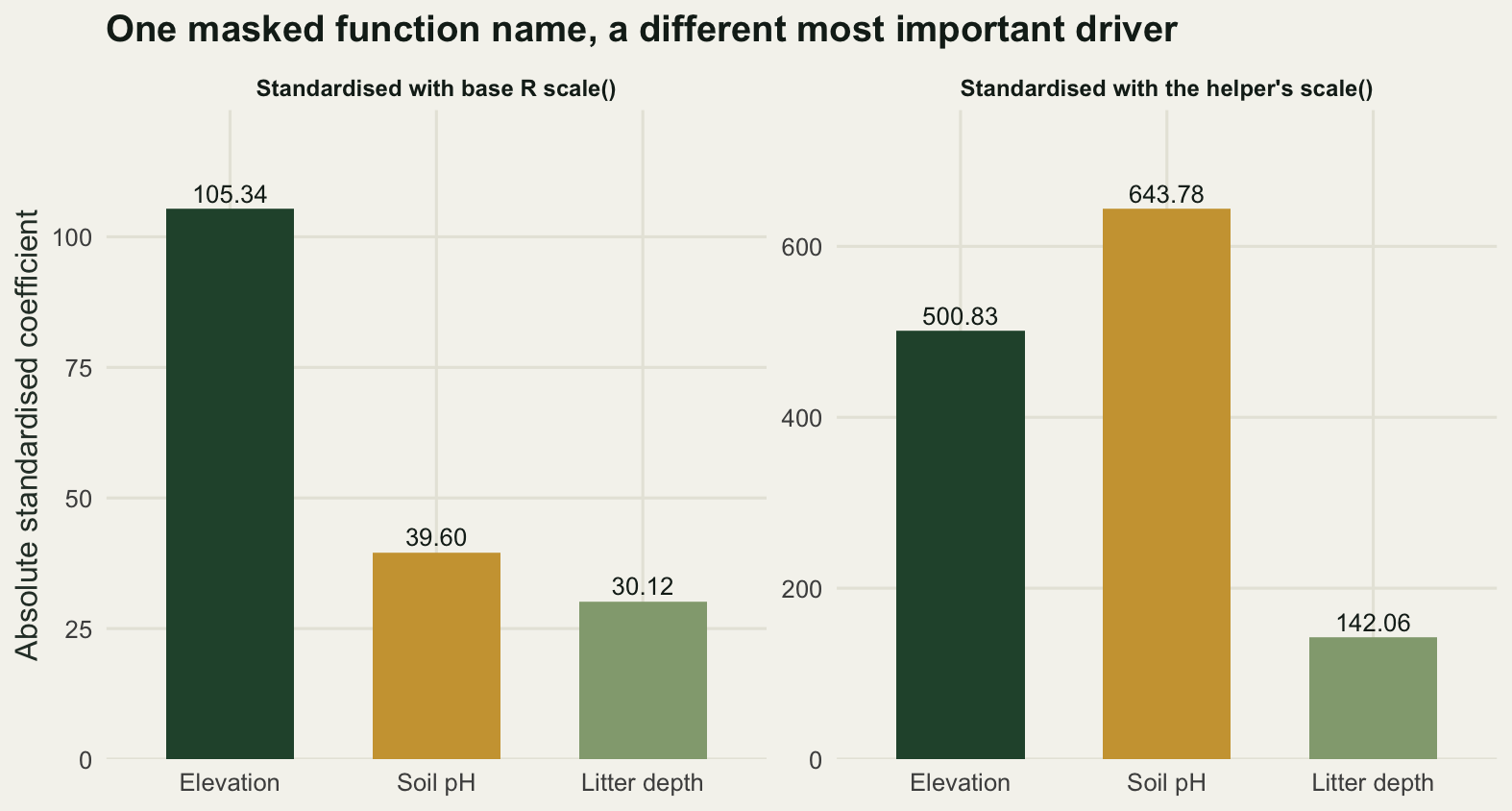
The honest limit
A package is not free, and the sections above have measured only one side of the ledger. The other side is the time it takes to build and keep one, and whether that time is repaid depends on how many analyses share the code and on what a wrong number costs you when it is found.
The calculation below stipulates its costs in minutes. They are not measured; they are a set of figures a working ecologist can argue with, and arguing with them is the point. Building the first package takes an afternoon. Each edit afterwards costs a documentation and check cycle rather than a one-line change. Copying a file into another project is quick. Discovering that a published number came out of a stale copy is expensive, because it means re-running the analysis, re-checking the figures and, in the bad case, writing to an editor.
setup_pkg  <- 210   # DESCRIPTION, NAMESPACE, a help page, the first check
reuse_pkg  <- 2     # one library() call in a new analysis
edit_pkg   <- 15    # edit, re-document, re-check, reinstall
reuse_copy <- 6     # copy the file in and fix the paths
edit_copy  <- 4     # per other copy, when you remember
repair     <- 240   # tracing one stale result after the fact

cost_pkg  <- function(n) setup_pkg + n * reuse_pkg + k_edit * edit_pkg
cost_copy <- function(n, p, fix) n * reuse_copy + k_edit * edit_copy * (n - 1) +
  fix * n * (1 - q_one(n, p)^k_edit)
breakeven <- function(fix, p = 0.5) {
  n <- 1:60
  d <- sapply(n, function(m) cost_pkg(m) - cost_copy(m, p, fix))
  if (all(d > 0)) NA_integer_ else n[which(d <= 0)][1]
}
round(c(package_cost_minutes_at_three_analyses = cost_pkg(3),
        copy_cost_minutes_at_three_analyses = cost_copy(3, 0.5, repair),
        copy_cost_minutes_at_three_ignoring_drift = cost_copy(3, 0.5, 0),
        expected_stale_copies_of_three = 3 * (1 - q_one(3, 0.5)^k_edit),
        breakeven_analyses_if_drift_costs_nothing = breakeven(0),
        breakeven_analyses_if_a_stale_result_costs_an_hour = breakeven(60),
        breakeven_analyses_if_a_stale_result_costs_four_hours =
          breakeven(repair)), 4)
package_cost_minutes_at_three_analyses
276.0000
copy_cost_minutes_at_three_analyses
627.7778
copy_cost_minutes_at_three_ignoring_drift
50.0000
expected_stale_copies_of_three
2.4074
breakeven_analyses_if_drift_costs_nothing
15.0000
breakeven_analyses_if_a_stale_result_costs_an_hour
5.0000
breakeven_analyses_if_a_stale_result_costs_four_hours
2.0000 Read that as a range rather than a threshold. If a stale copy costs nothing, because nobody ever finds out, the package pays from the 15th analysis and you should not write one for two projects. If a stale copy costs an hour to trace, it pays from the 5th. If it costs four hours, which is a modest estimate for a number that has already been sent out, it pays from the 2nd. The variable that moves the answer is not the cost of the package. It is what you believe about the consequences of a wrong number, and that belief is not something a measurement in this post can settle for you.
Four other limits are worth stating plainly.
The measurement here is about drift between copies, not about whether the shared version is right. Every number in the first half of this post compares an analysis against the shared source, and the shared source is only correct because this survey was simulated and the correct definition is known. In your project it is a version somebody decided on. A package makes one definition authoritative; it does not make it true.
A package pins nothing outside itself. Imports: stats records that cpue needs stats; it does not record which version of stats, which version of R, or which BLAS the machine had, and a default that changes in a dependency will change your results in exactly the silent way the first section described. That is the job of a lockfile, which is pinning package versions with renv.
R CMD check is not a correctness check. It verifies that the package installs, that the examples run, that the documentation matches the arguments and that the tests you wrote pass. If your tests are thin, a green check means the package is well formed and says nothing about the function.
And the version number in DESCRIPTION is a promise a human has to keep. Nothing in R stops you editing R/cpue.R, reinstalling, and leaving the version at 0.4.0, at which point you have a package whose identity lies about its contents. The 16 versions counted earlier can happen inside a package too. What the package changes is that there is now one place to look, and one number to increment when it changes.
Where to go next
The moment the helper is shared, changing it becomes riskier than changing a copy, because one edit now reaches every analysis. Testing your analysis code writes the suite that makes that safe, and it is the same tests/testthat/ directory the package layout above already has a slot for. Debugging and defensive R code covers what to put at the top of a shared function so that a caller who passes the wrong thing is told straight away rather than three steps later.
For everything around the package, a reproducible statistical workflow in R puts the pieces in order, pinning package versions with renv records what your package was built against, and git for ecologists answers the question this post keeps skirting: not which copy is current, but which state of the code produced the figure that is now in the manuscript.
References
Wilson G, Bryan J, Cranston K, Kitzes J, Nederbragt L, Teal TK 2017 PLoS Computational Biology 13(6):e1005510 (10.1371/journal.pcbi.1005510)
Wickham H, Bryan J 2023 R Packages, 2nd edition, O’Reilly Media (ISBN 978-1-0981-3494-5)
Marwick B, Boettiger C, Mullen L 2018 The American Statistician 72(1):80-88 (10.1080/00031305.2017.1375986)
Peng RD 2011 Science 334(6060):1226-1227 (10.1126/science.1213847)
Sandve GK, Nekrutenko A, Taylor J, Hovig E 2013 PLoS Computational Biology 9(10):e1003285 (10.1371/journal.pcbi.1003285)