library(ggplot2)

te_pal <- list(forest = "#275139", green = "#2f8f63", sage = "#93a87f",
               clay = "#b5534e", gold = "#cda23f", line = "#dad9ca",
               ink = "#16241d", paper = "#f5f4ee")

theme_te <- function() {
  theme_minimal(base_size = 12) +
    theme(panel.grid.minor = element_blank(),
          panel.grid.major = element_line(colour = "#e7e6dc"),
          plot.background = element_rect(fill = "#f5f4ee", colour = NA),
          panel.background = element_rect(fill = "#f5f4ee", colour = NA),
          plot.title = element_text(face = "bold", colour = te_pal$ink),
          axis.title = element_text(colour = "#2c3a31"))
}Debugging and defensive R code
R
reproducibility
ecology tutorial
ggplot2
The expensive R error is the one that runs and returns a wrong number. Measured on a beetle survey: what stays silent, what it costs, and what catches it.
An analysis of pitfall trap data stops with a message about contrasts. You have never written the word contrasts in your life. You read the message three times, work out which line it came from, and find that the line is fine: it fits a linear model to twelve site means, which is what it is supposed to do. The fault is seven stages upstream, in a lookup that returned nothing because a column was called code and the script asked for site.
That error cost an afternoon and it is the cheap one, because it stopped. In the same script two other things went wrong. One of them warned, which meant it announced itself in a way that is easy to scroll past. The third neither stopped nor warned. It produced a table of the right shape with plausible numbers in it, and the grazing effect it reported was 62 per cent larger than the truth.
This post measures the three of them on the same analysis. It then takes the silent one apart, because vector recycling is a common mechanism behind silent arithmetic errors in R, and it does its worst damage in exactly the balanced designs that good field practice produces. After that comes the other silent error that nobody warns ecologists about: a numeric covariate that arrives as a factor, where as.numeric returns the level index rather than the value. The last section prices the defence. Twelve clauses of precondition checking at the top of one function, scored against ten faults, against what R says by itself and against what tryCatch adds.
The survey and the number it reports
Twelve grassland sites, six grazed and six ungrazed, each visited five times with pitfall traps. Every record carries the site, the visit, the number of trap nights the trap was open and the beetle catch. A separate table holds one detection correction weight per site, the kind of adjustment that comes from a vegetation height model or a paired mark-recapture calibration. The analysis standardises each catch to a rate per hundred trap nights, multiplies by the site weight, averages up to the site, and reports the percentage by which the grazed sites exceed the ungrazed ones.
set.seed(20260811)

n_site  <- 12
n_visit <- 5
site  <- sprintf("S%02d", 1:n_site)
treat <- rep(c("grazed", "ungrazed"), each = 6)

d <- data.frame(site = rep(site, each = n_visit),
                visit = rep(1:n_visit, times = n_site),
                stringsAsFactors = FALSE)
d$treat  <- treat[match(d$site, site)]
d$nights <- sample(4:10, nrow(d), replace = TRUE)
site_rate <- ifelse(treat == "grazed", 3.6, 2.4) * exp(rnorm(n_site, 0, 0.18))
d$catch  <- rpois(nrow(d), site_rate[match(d$site, site)] * d$nights)

wt <- data.frame(code = site, weight = round(runif(n_site, 0.75, 1.45), 3),
                 stringsAsFactors = FALSE)
w <- wt$weight
names(w) <- wt$code

analyse <- function(recs, wvec) {
  rate <- 100 * recs$catch / recs$nights
  corr <- rate * wvec
  sm <- tapply(corr, recs$site, mean)
  tb <- data.frame(site = names(sm), treat = treat[match(names(sm), site)],
                   mean_rate = as.numeric(sm), stringsAsFactors = FALSE)
  fit <- lm(mean_rate ~ treat, data = tb)
  100 * -coef(fit)[[2]] / mean(tb$mean_rate[tb$treat == "ungrazed"])
}

base_recs <- d[, c("site", "visit", "treat", "nights", "catch")]
base_w <- as.numeric(w[d$site])
site_mean <- tapply(100 * d$catch / d$nights * base_w, d$site, mean)
true_effect <- analyse(base_recs, base_w)

print(head(d, 4))
site visit treat nights catch
1 S01 1 grazed 4 12
2 S01 2 grazed 4 15
3 S01 3 grazed 9 32
4 S01 4 grazed 8 25print(wt) code weight
1 S01 0.858
2 S02 0.801
3 S03 1.087
4 S04 0.935
5 S05 1.244
6 S06 0.917
7 S07 1.206
8 S08 1.229
9 S09 0.762
10 S10 1.284
11 S11 1.081
12 S12 0.868round(c(records = nrow(d), sites = n_site, visits_per_site = n_visit,
analysis_lines = length(deparse(analyse)),
reported_grazing_effect_percent = true_effect), 4) records sites
60.0000 12.0000
visits_per_site analysis_lines
5.0000 10.0000
reported_grazing_effect_percent
22.5741 The number the paper would carry is 22.5741 per cent. That is not the contrast the generator was given; it is what the correct code returns once the per-site weights have landed where they landed, and everything that follows is a comparison against it, which is the only reference a bug hunt needs. The unit for all the damage measurements below is a percentage point of that reported effect, which keeps the comparison honest: a fault that moves the answer by a tenth of a point and a fault that moves it by twenty are not the same problem, even if both are wrong.
Three errors, and what each one costs to find
Write the analysis out as eight named stages, each one taking the previous result and producing the next. That is what the script is anyway; naming the stages just makes the intermediate values addressable, which is the first thing you need when something goes wrong.
d$nights_txt <- as.character(d$nights)
bad_rows <- c(9, 28, 47)

stage_names <- c("weights", "nights", "usable", "rate",
                 "corrected", "site means", "site table", "contrast")

run_pipe <- function(fault = "none", guarded = FALSE) {
  dd <- d
  if (fault == "text nights") dd$nights_txt[bad_rows] <- "not set"
  vals <- vector("list", 8)
  names(vals) <- stage_names
  log <- data.frame(stage = integer(0), kind = character(0), text = character(0),
                    stringsAsFactors = FALSE)
  stopped <- FALSE
  step <- function(i, expr) {
    if (stopped) return(NULL)
    v <- withCallingHandlers(
      tryCatch(expr, error = function(e) {
        log <<- rbind(log, data.frame(stage = i, kind = "error",
                                      text = conditionMessage(e),
                                      stringsAsFactors = FALSE))
        stopped <<- TRUE
        NULL
      }),
      warning = function(w) {
        log <<- rbind(log, data.frame(stage = i, kind = "warning",
                                      text = conditionMessage(w),
                                      stringsAsFactors = FALSE))
        invokeRestart("muffleWarning")
      })
    vals[[i]] <<- v
    v
  }

  wv <- step(1, {
    v <- if (fault == "missing column") wt$weight[match(dd$site, wt$site)]
         else wt$weight[match(dd$site, wt$code)]
    if (guarded) stopifnot(length(v) == nrow(dd), all(is.finite(v)))
    v })
  ni <- step(2, {
    v <- as.numeric(dd$nights_txt)
    if (guarded) stopifnot(all(is.finite(v)), all(v > 0))
    v })
  us <- step(3, { dd$nights <- ni; dd$w <- wv; dd[ni > 0, ] })
  ra <- step(4, 100 * us$catch / us$nights)
  co <- step(5, {
    wvec <- if (fault == "recycled") wt$weight else us$w
    if (guarded) stopifnot(length(wvec) == nrow(us))
    ra * wvec })
  sm <- step(6, tapply(co, us$site, mean))
  tb <- step(7, data.frame(site = names(sm), treat = treat[match(names(sm), site)],
                           mean_rate = as.numeric(sm), stringsAsFactors = FALSE))
  ef <- step(8, {
    fit <- lm(mean_rate ~ treat, data = tb)
    100 * -coef(fit)[[2]] / mean(tb$mean_rate[tb$treat == "ungrazed"])
  })
  list(vals = vals, log = log, effect = if (is.null(ef)) NA_real_ else ef)
}

clean <- run_pipe("none")
round(c(stages = length(stage_names),
        messages_on_the_clean_run = nrow(clean$log),
        effect_on_the_clean_run = clean$effect), 4)
stages messages_on_the_clean_run effect_on_the_clean_run
8.0000 0.0000 22.5741 Three faults go in, one at a time. The first is the column name: wt$site instead of wt$code. There is no such column, so $ returns NULL, match against NULL returns missing for every record, and the weight vector comes back as sixty missing values. R says nothing at the time. The second is a trap nights column that arrived as text, with three cells reading not set; as.numeric turns those into missing values and warns while doing it. The third is the recycled weight vector, the subject of the next section, which produces no message of any kind.
locate <- function(x) {
  if (is.null(x) || length(x) == 0) return("nothing there")
  num <- if (is.data.frame(x)) unlist(x[vapply(x, is.numeric, logical(1))]) else
         if (is.numeric(x)) x else NULL
  if (!is.null(num) && length(num) > 0) {
    if (anyNA(num)) return("missing values")
    if (any(!is.finite(num))) return("not finite")
    if (any(num < 0)) return("negative")
  }
  NA_character_
}

fault_names <- c("missing column", "text nights", "recycled")
fault_stage <- c(1, 2, 5)

scan_one <- function(f) {
  r <- run_pipe(f)
  g <- run_pipe(f, guarded = TRUE)
  flags <- vapply(r$vals[1:7], locate, character(1))
  hit <- which(!is.na(flags))
  data.frame(fault = f,
             r_kind = if (nrow(r$log)) r$log$kind[1] else "silence",
             r_stage = if (nrow(r$log)) r$log$stage[1] else NA_integer_,
             fault_stage = fault_stage[match(f, fault_names)],
             inspected = if (length(hit)) hit[1] else 7L,
             found = length(hit) > 0,
             guard_stage = if (nrow(g$log)) g$log$stage[1] else NA_integer_,
             effect = r$effect, stringsAsFactors = FALSE)
}
scan <- do.call(rbind, lapply(fault_names, scan_one))
scan$gap <- scan$r_stage - scan$fault_stage
scan$shift <- scan$effect - true_effect
print(scan, right = FALSE)
fault r_kind r_stage fault_stage inspected found guard_stage
weights missing column error 8 1 1 TRUE 1
nights text nights warning 2 2 2 TRUE 2
1 recycled silence NA 5 7 FALSE 5
effect gap shift
weights NA 7 NA
nights 26.49815 0 3.924041
1 36.67264 NA 14.098534for (f in fault_names) {
lg <- run_pipe(f)$log
cat(f, ":", if (nrow(lg)) paste0(lg$kind[1], " at stage ", lg$stage[1], ", ",
lg$text[1]) else "no message at all", "\n")
}missing column : error at stage 8, contrasts can be applied only to factors with 2 or more levels
text nights : warning at stage 2, NAs introduced by coercion
recycled : no message at all round(c(stages_between_message_and_fault_missing_column = scan$gap[1],
stages_between_message_and_fault_text_nights = scan$gap[2],
intermediates_inspected_missing_column = scan$inspected[1],
intermediates_inspected_text_nights = scan$inspected[2],
intermediates_inspected_recycled = scan$inspected[3],
faults_a_scan_of_the_intermediates_finds = sum(scan$found),
reported_effect_text_nights_percent = scan$effect[2],
reported_effect_recycled_percent = scan$effect[3],
shift_text_nights_points = scan$shift[2],
shift_recycled_points = scan$shift[3]), 4)stages_between_message_and_fault_missing_column
7.0000
stages_between_message_and_fault_text_nights
0.0000
intermediates_inspected_missing_column
1.0000
intermediates_inspected_text_nights
2.0000
intermediates_inspected_recycled
7.0000
faults_a_scan_of_the_intermediates_finds
2.0000
reported_effect_text_nights_percent
26.4981
reported_effect_recycled_percent
36.6726
shift_text_nights_points
3.9240
shift_recycled_points
14.0985 fl <- c("Missing column name", "Trap nights as text", "Recycled weights")
row_of <- c(3, 2, 1)
marker <- c("Where the fault is", "Where R's message points",
"Where a precondition stops the run")
off <- c(0.19, 0, -0.19)
map_df <- data.frame(
row = rep(row_of, each = 3) + rep(off, 3),
what = factor(rep(marker, 3), levels = marker),
stage = c(scan$fault_stage[1], scan$r_stage[1], scan$guard_stage[1],
scan$fault_stage[2], scan$r_stage[2], scan$guard_stage[2],
scan$fault_stage[3], NA, scan$guard_stage[3]))
map_df <- map_df[!is.na(map_df$stage), ]
gap_df <- data.frame(x = scan$fault_stage[1], y = row_of[1] + off[1],
xend = scan$r_stage[1], yend = row_of[1] + off[2])
note_df <- data.frame(stage = 6.2, row = row_of[3],
lab = "R says nothing at all")
ggplot(map_df, aes(stage, row)) +
geom_segment(data = gap_df, aes(x = x, xend = xend, y = y, yend = yend),
inherit.aes = FALSE, colour = te_pal$sage, linewidth = 1.4,
arrow = arrow(length = unit(8, "pt"), type = "closed")) +
geom_point(aes(shape = what, colour = what), size = 4.4, stroke = 1.3) +
geom_text(data = note_df, aes(stage, row, label = lab), inherit.aes = FALSE,
colour = te_pal$clay, size = 3.5, hjust = 0, fontface = "italic") +
scale_shape_manual(values = c(16, 17, 0), name = NULL) +
scale_colour_manual(values = c(te_pal$forest, te_pal$clay, te_pal$gold),
name = NULL) +
scale_x_continuous(breaks = 1:8, labels = stage_names, limits = c(0.7, 8.7)) +
scale_y_continuous(breaks = row_of, labels = fl, limits = c(0.5, 3.5)) +
labs(x = "Analysis stage", y = NULL,
title = "Only one of the three faults is reported where it happens") +
theme_te() +
theme(legend.position = "top",
panel.grid.major.y = element_blank(),
axis.text.x = element_text(size = 8.5),
axis.text.y = element_text(size = 10, colour = te_pal$ink),
legend.text = element_text(size = 9))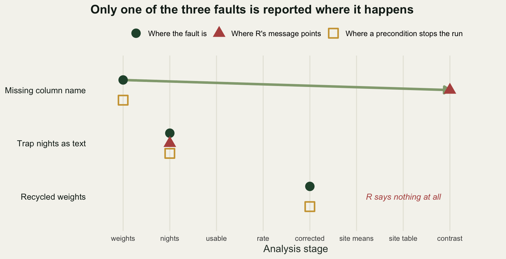
The missing column name is the loudest fault and the least helpful message. R stops at stage 8 with contrasts can be applied only to factors with 2 or more levels, which is a statement about model matrices, and the fault is at stage 1, 7 stages away. Nothing on the way there complains, because a vector of missing values is a perfectly legal thing to divide, multiply and average.
The trap nights column is the polite one. The warning comes from stage 2, which is where the fault is, so the distance is 0. It costs 2 inspections of intermediate values to confirm. The analysis then finishes and reports 26.4981 per cent, which is 3.9240 points off the truth, because three records dropped out and they were not a random three.
The recycled weights get no message, and that is the finding. A scan of the intermediates does not help either. The rule used here is the one a human eye applies when it stares at an object in the console: is anything missing, is anything not finite, is anything negative where it cannot be. That rule flags the first fault at the first intermediate and the second at the second. On the recycled run it flags nothing at all, across every one of the 7 intermediate values, because every one of them is the right length and full of positive finite numbers. Only 2 of the 3 faults are findable by looking. The answer that comes out the far end is 36.6726 per cent against a true 22.5741.
The precondition column is the answer to that, and it is worth noticing what it does to the first fault as well as the third. With a stopifnot at the head of each stage the missing column stops at stage 1 instead of stage 8, and the recycled weights stop at stage 5 instead of never. In all three cases the message arrives where the fault is. The next three sections work out what those checks are worth and what they cost.
The silent one: R recycles a short vector without asking
R’s recycling rule is that an arithmetic operation between vectors of different lengths repeats the shorter one until it is as long as the longer one. It is a genuinely useful rule: counts / 2 and counts - mean(counts) both depend on it. It is also the reason rate * w runs when rate has one element per record and w has one element per site.
The survey has 60 records and 12 sites. Sixty is a multiple of twelve, so R has no complaint to make. The weights simply march through the record vector in a twelve step cycle while the records march through in five step blocks, and the two cycles agree only where they happen to coincide.
rate <- 100 * d$catch / d$nights
correct <- rate * base_w
recycled <- rate * wt$weight

due <- match(d$site, site)
applied <- ((seq_len(nrow(d)) - 1) %% n_site) + 1
align <- data.frame(record = 1:14, site = d$site[1:14],
                    weight_due = wt$weight[due[1:14]],
                    weight_applied = wt$weight[applied[1:14]],
                    right = due[1:14] == applied[1:14])
print(align, right = FALSE)
record site weight_due weight_applied right
1 1 S01 0.858 0.858 TRUE
2 2 S01 0.858 0.801 FALSE
3 3 S01 0.858 1.087 FALSE
4 4 S01 0.858 0.935 FALSE
5 5 S01 0.858 1.244 FALSE
6 6 S02 0.801 0.917 FALSE
7 7 S02 0.801 1.206 FALSE
8 8 S02 0.801 1.229 FALSE
9 9 S02 0.801 0.762 FALSE
10 10 S02 0.801 1.284 FALSE
11 11 S03 1.087 1.081 FALSE
12 12 S03 1.087 0.868 FALSE
13 13 S03 1.087 0.858 FALSE
14 14 S03 1.087 0.801 FALSEsm_rec <- tapply(recycled, d$site, mean)
site_err <- 100 * (sm_rec / site_mean - 1)
eff_rec <- analyse(base_recs, wt$weight)
pair_flip <- function(a, b) {
ij <- which(upper.tri(matrix(0, length(a), length(a))), arr.ind = TRUE)
100 * mean(sign(a[ij[, 1]] - a[ij[, 2]]) * sign(b[ij[, 1]] - b[ij[, 2]]) < 0)
}
round(c(records = nrow(d),
records_given_the_right_weight = sum(due == applied),
sites_moved_more_than_ten_percent = sum(abs(site_err) > 10),
worst_site_error_percent = max(abs(site_err)),
grand_mean_error_percent = 100 * (mean(sm_rec) / mean(site_mean) - 1),
site_pairs = choose(n_site, 2),
pairs_reversed_percent = pair_flip(site_mean, sm_rec),
true_effect_percent = true_effect,
recycled_effect_percent = eff_rec,
shift_in_points = eff_rec - true_effect,
relative_inflation_percent = 100 * (eff_rec / true_effect - 1)), 4) records records_given_the_right_weight
60.0000 8.0000
sites_moved_more_than_ten_percent worst_site_error_percent
9.0000 45.1890
grand_mean_error_percent site_pairs
2.8883 66.0000
pairs_reversed_percent true_effect_percent
33.3333 22.5741
recycled_effect_percent shift_in_points
36.6726 14.0985
relative_inflation_percent
62.4545 print(round(site_err, 2)) S01 S02 S03 S04 S05 S06 S07 S08 S09 S10 S11
16.76 38.94 -11.60 18.45 -21.74 7.56 -7.50 -24.99 45.19 -23.33 -0.74
S12
17.67 Of the 60 records, 8 get the weight that belongs to their own site. The other 52 get a weight belonging to some other site, and nothing anywhere in the run says so.
The consequence is not spread evenly and that is what makes it dangerous. The grand mean of the twelve site means is out by 2.8883 per cent, which is inside the noise of anything you would notice by looking at the total. The worst individual site is out by 45.1890 per cent, 9 of the 12 sites move by more than 10 per cent, and 33.3333 per cent of the 66 site pairs come out ranked the wrong way round. The aggregate looks fine because the weights are conserved: every weight is used five times, just against the wrong records, so the sum is nearly preserved while the allocation is destroyed.
The reported grazing effect goes from 22.5741 per cent to 36.6726 per cent, a shift of 14.0985 points and a relative inflation of 62.4545 per cent. The direction survives, which is the worst possible outcome, because a result that changes sign gets questioned and a result that keeps its direction gets written up whatever its size.
rec_df <- data.frame(
  site = factor(rep(names(site_mean), 2), levels = rev(names(site_mean))),
  treat = rep(treat, 2),
  value = c(as.numeric(site_mean), as.numeric(sm_rec)),
  version = factor(rep(c("Each site's own weight", "Weights recycled"),
                       each = n_site),
                   levels = c("Each site's own weight", "Weights recycled")))
seg_df <- data.frame(site = factor(names(site_mean),
                                   levels = rev(names(site_mean))),
                     treat = treat, lo = pmin(site_mean, sm_rec),
                     hi = pmax(site_mean, sm_rec))

ggplot(rec_df, aes(value, site)) +
  geom_segment(data = seg_df, aes(x = lo, xend = hi, y = site, yend = site),
               inherit.aes = FALSE, colour = te_pal$line, linewidth = 2.4) +
  geom_point(aes(colour = version, shape = version), size = 3.2, stroke = 1.2) +
  facet_grid(treat ~ ., scales = "free_y", space = "free_y") +
  scale_colour_manual(values = c(te_pal$forest, te_pal$clay), name = NULL) +
  scale_shape_manual(values = c(16, 1), name = NULL) +
  labs(x = "Mean corrected catch per hundred trap nights", y = NULL,
       title = "Recycled weights move nine of the twelve site means by over ten per cent") +
  theme_te() +
  theme(legend.position = "top",
        strip.text = element_text(colour = te_pal$ink, face = "bold", size = 9))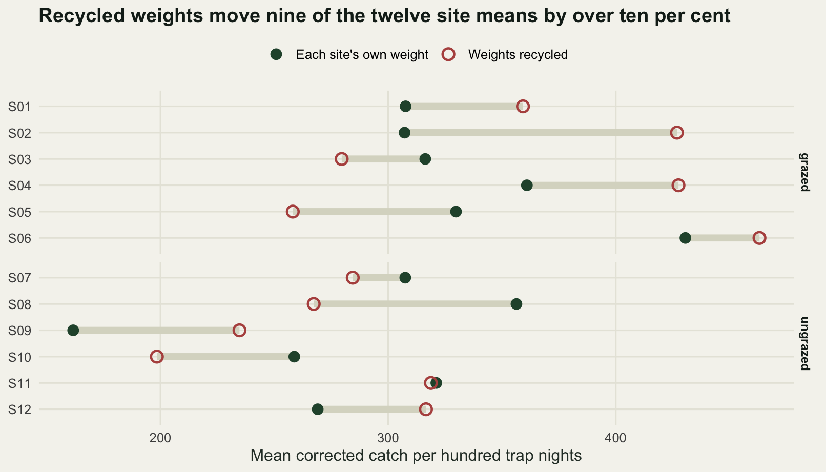
Now the near miss. Lose one trap, so that 59 records are left, and 59 is not a multiple of 12. R then warns: longer object length is not a multiple of shorter object length. The identical mistake, made against slightly messier data, announces itself.
ragged <- base_recs[-7, ]
caught <- character(0)
rag_rec <- withCallingHandlers(
  analyse(ragged, wt$weight),
  warning = function(w) {
    caught <<- c(caught, conditionMessage(w))
    invokeRestart("muffleWarning")
  })
rag_true <- analyse(ragged, as.numeric(w[ragged$site]))
rag_due <- match(ragged$site, site)
rag_applied <- ((seq_len(nrow(ragged)) - 1) %% n_site) + 1

cat("warning:", caught, "\n")
warning: longer object length is not a multiple of shorter object length round(c(records_after_the_loss = nrow(ragged),
is_a_multiple_of_twelve = nrow(d) %% n_site,
remainder_after_the_loss = nrow(ragged) %% n_site,
records_given_the_right_weight = sum(rag_due == rag_applied),
true_effect_on_these_records = rag_true,
recycled_effect_on_these_records = rag_rec,
shift_in_points = rag_rec - rag_true,
warnings_raised = length(caught)), 4) records_after_the_loss is_a_multiple_of_twelve
59.0000 0.0000
remainder_after_the_loss records_given_the_right_weight
11.0000 4.0000
true_effect_on_these_records recycled_effect_on_these_records
22.3777 35.1969
shift_in_points warnings_raised
12.8193 1.0000 The ragged version does the same kind of damage: 4 of the 59 records get the right weight and the reported effect moves from 22.3777 to 35.1969, a shift of 12.8193 points. It also raises exactly 1 warning, and the balanced version raises none.
That is worth stating plainly, because it inverts the usual advice. The warning is a statement about arithmetic, not about correctness. It appears when the lengths do not divide, and a balanced design with an equal number of visits at every site is precisely the case where they do. Run the same bug on a complete, tidy, well-organised data set and R is silent. Run it on a data set with a flooded trap in it and R speaks up. The better your fieldwork, the quieter the mistake.
The fix is to stop relying on position and carry the key. w[d$site] is a lookup by site code, so a missing code gives that record an NA rather than quietly reusing whatever is next in line. The failure stays silent, but it leaves a missing value you can test for instead of a plausible wrong number. merge on the code column matches on the same key at the data frame level. When you have written the lookup, one line confirms it worked:
wv <- w[d$site]
round(c(length_matches_records = as.numeric(length(wv) == nrow(d)),
        every_record_has_a_weight = as.numeric(!anyNA(wv)),
        every_record_has_its_own_sites_weight =
          as.numeric(all(wv == w[d$site])),
        weights_that_differ_from_the_recycled_version =
          sum(as.numeric(wv) != wt$weight[applied])), 4)
length_matches_records
1
every_record_has_a_weight
1
every_record_has_its_own_sites_weight
1
weights_that_differ_from_the_recycled_version
52 A numeric column that arrived as a factor
Thirty sites on an elevation gradient from the valley floor to the ridge, with species richness falling as you climb. The elevation column came off a spreadsheet as text rather than as numbers, and somewhere in the import it became a factor. The analyst writes as.numeric(elevation) and fits the regression.
as.numeric on a factor does not return the values. It returns the integer codes: the position of each value in the level table. The level table is sorted, and it is sorted as text, so the order it produces is the dictionary order of the printed numbers rather than their numeric order.
set.seed(20260811)
n_elev <- 30
elev <- round(runif(n_elev, 60, 1450))
rich <- round(26 - 0.011 * elev + rnorm(n_elev, 0, 1.8))
sheet <- as.character(elev)
f <- factor(sheet)
idx <- as.numeric(f)

cat("first eight levels in level order:", levels(f)[1:8], "\n")
first eight levels in level order: 1032 1048 1071 1073 1088 1115 1130 1135 cat("the same eight elevations sorted numerically:",
sort(elev)[1:8], "\n")the same eight elevations sorted numerically: 69 119 295 329 342 390 463 580 fit_stats <- function(fit) {
cf <- summary(fit)$coefficients
c(slope = cf[2, 1], p_value = cf[2, 4], r_squared = summary(fit)$r.squared)
}
fit_true <- lm(rich ~ elev)
fit_idx <- lm(rich ~ idx)
round(c(sites = n_elev, levels = nlevels(f),
lowest_site_m = min(elev), highest_site_m = max(elev),
gradient_span_m = diff(range(elev)),
spearman_index_against_elevation = cor(idx, elev, method = "spearman"),
index_runs_from = min(idx), index_runs_to = max(idx)), 4) sites levels
30.0000 28.0000
lowest_site_m highest_site_m
69.0000 1438.0000
gradient_span_m spearman_index_against_elevation
1369.0000 -0.4796
index_runs_from index_runs_to
1.0000 28.0000 round(c(true_slope_species_per_metre = fit_stats(fit_true)[1],
true_p_value = fit_stats(fit_true)[2],
true_r_squared = fit_stats(fit_true)[3],
index_slope_species_per_level = fit_stats(fit_idx)[1],
index_p_value = fit_stats(fit_idx)[2],
index_r_squared = fit_stats(fit_idx)[3]), 6) true_slope_species_per_metre.slope true_p_value.p_value
-0.010679 0.000000
true_r_squared.r_squared index_slope_species_per_level.slope
0.846339 0.265723
index_p_value.p_value index_r_squared.r_squared
0.009291 0.218003 round(c(true_richness_change_over_the_gradient =
coef(fit_true)[[2]] * diff(range(elev)),
index_richness_change_over_the_gradient =
coef(fit_idx)[[2]] * (nlevels(f) - 1),
recovered_by_as_numeric_as_character =
max(abs(as.numeric(as.character(f)) - elev))), 4) true_richness_change_over_the_gradient index_richness_change_over_the_gradient
-14.6197 7.1745
recovered_by_as_numeric_as_character
0.0000 The level order is the first surprise. The eight lowest levels are all four digit elevations starting with a one, because "1032" sorts before "69" for the same reason "apple" sorts before "zebra". The rank correlation between the level index and the actual elevation is -0.4796, so the covariate is not merely rescaled, it is scrambled.
The regression says what you would expect from that. The true fit gives a slope of -0.010679 species per metre with a p value that rounds to 0 at six decimal places, which over the 1369 metres between the lowest and the highest site is a loss of 14.6197 species. The fit on the level index gives a slope of +0.265723 species per level with a p value of 0.009291, which on this run clears the conventional five per cent threshold and has the wrong sign. Read as a gradient it claims a gain of 7.1745 species from the valley to the ridge. The elevation effect in these data is real, large and downhill, and the broken analysis has turned it into an uphill increase.
Now the version that should worry you more. Restrict the analysis to the sites between 100 and 999 metres. Every elevation is now three characters wide, so the dictionary order of the strings is the numeric order of the values, and the level index becomes the rank of the elevation. Nothing is shuffled any more.
k <- elev >= 100 & elev <= 999
f2 <- factor(as.character(elev[k]))
idx2 <- as.numeric(f2)
fit_t2 <- lm(rich[k] ~ elev[k])
fit_i2 <- lm(rich[k] ~ idx2)

round(c(sites_in_the_window = sum(k),
        spearman_index_against_elevation = cor(idx2, elev[k], method = "spearman"),
        lowest_m = min(elev[k]), highest_m = max(elev[k])), 4)
sites_in_the_window spearman_index_against_elevation
14 1
lowest_m highest_m
119 979 round(c(true_slope_species_per_metre = fit_stats(fit_t2)[1],
true_p_value = fit_stats(fit_t2)[2],
true_r_squared = fit_stats(fit_t2)[3],
index_slope_species_per_level = fit_stats(fit_i2)[1],
index_p_value = fit_stats(fit_i2)[2],
index_r_squared = fit_stats(fit_i2)[3]), 6) true_slope_species_per_metre.slope true_p_value.p_value
-0.009781 0.000039
true_r_squared.r_squared index_slope_species_per_level.slope
0.768425 -0.595604
index_p_value.p_value index_r_squared.r_squared
0.000025 0.784082 round(c(true_richness_change = coef(fit_t2)[[2]] * diff(range(elev[k])),
index_richness_change = coef(fit_i2)[[2]] * (nlevels(f2) - 1),
error_in_the_reported_gradient_percent =
100 * (coef(fit_i2)[[2]] * (nlevels(f2) - 1) /
(coef(fit_t2)[[2]] * diff(range(elev[k]))) - 1)), 4) true_richness_change index_richness_change
-8.4117 -7.7429
error_in_the_reported_gradient_percent
-7.9511 pn <- c("Elevation in metres\n(the column parsed)",
"Level index, all sites\n(mixed digit widths)",
"Level index, 100 to 999 m\n(equal digit widths)")
fac_df <- rbind(
data.frame(x = elev, y = rich, panel = pn[1]),
data.frame(x = idx, y = rich, panel = pn[2]),
data.frame(x = idx2, y = rich[k], panel = pn[3]))
fac_df$panel <- factor(fac_df$panel, levels = pn)
fac_fit <- data.frame(
intercept = c(coef(fit_true)[[1]], coef(fit_idx)[[1]], coef(fit_i2)[[1]]),
slope = c(coef(fit_true)[[2]], coef(fit_idx)[[2]], coef(fit_i2)[[2]]),
panel = factor(pn, levels = pn))
inner_breaks <- function(lims) {
pad <- 0.08 * diff(lims)
b <- pretty(lims, n = 5)
b[b > lims[1] + pad & b < lims[2] - pad]
}
ggplot(fac_df, aes(x, y)) +
geom_abline(data = fac_fit, aes(intercept = intercept, slope = slope),
colour = te_pal$clay, linewidth = 1) +
geom_point(colour = te_pal$forest, size = 2.4, alpha = 0.9) +
facet_wrap(~panel, scales = "free_x") +
scale_x_continuous(breaks = inner_breaks, expand = expansion(mult = 0.07)) +
labs(x = "Covariate as the model received it", y = "Species richness",
title = "The level index reverses the gradient, then hides inside a tidy window") +
theme_te() +
theme(panel.spacing.x = unit(1.4, "lines"),
panel.spacing.y = unit(16, "pt"),
strip.text = element_text(colour = te_pal$ink, face = "bold", size = 9))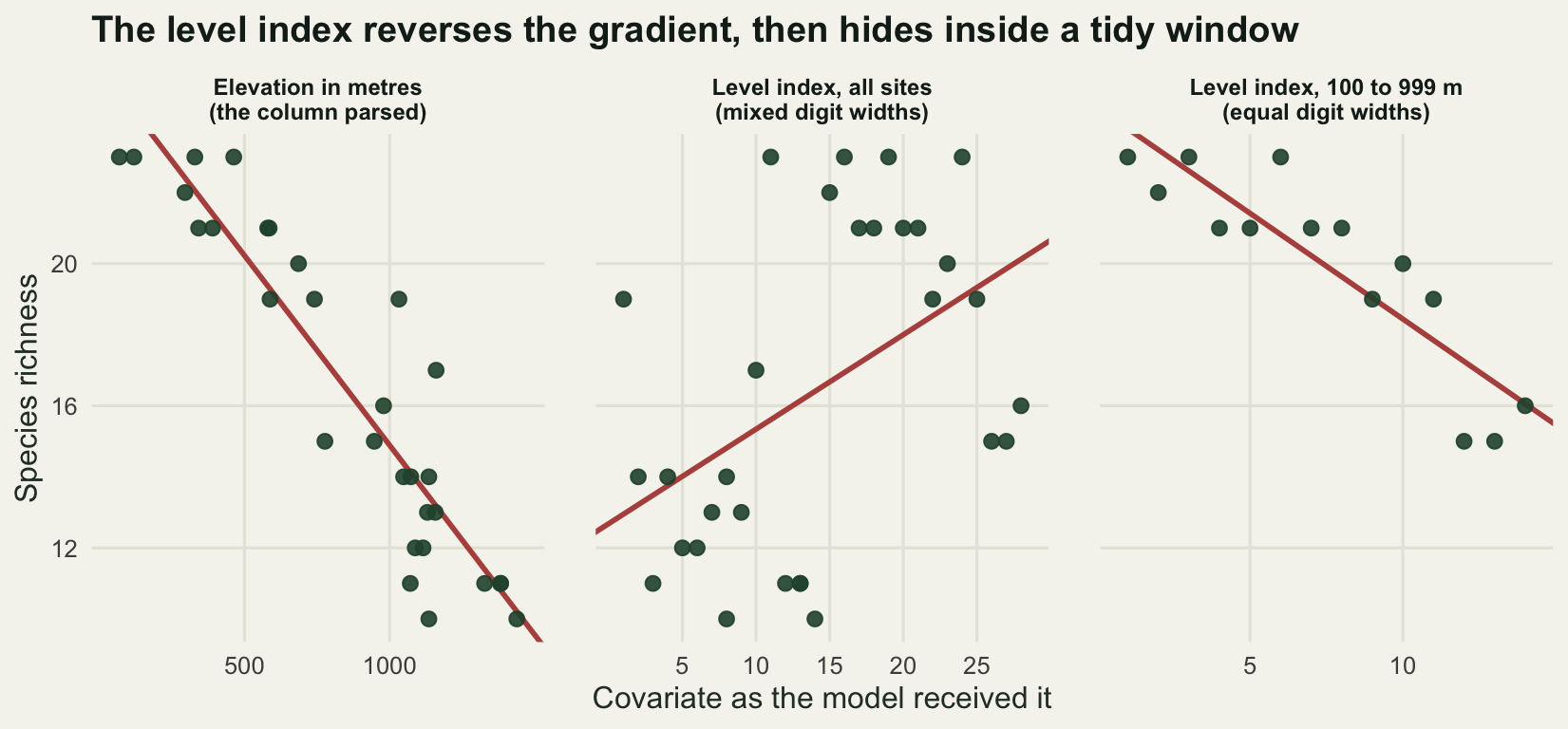
In that window the rank correlation between the index and the elevation is exactly 1. The true fit over the 14 sites gives -0.009781 species per metre with an r squared of 0.768425, and the index fit gives -0.595604 species per level with an r squared of 0.784082 and a p value just as small. Nothing in the diagnostics marks the broken model as the wrong one. The reported gradient, expressed as the richness change across the sampled range, is 7.7429 species against a true 8.4117, which is out by 7.9511 per cent.
That is the shape of the whole problem in one number. When the factor coding scrambles the covariate the analysis falls apart visibly and someone notices. When it does not scramble it, the analysis looks fine and reports a gradient that is wrong in units nobody can interpret, and there is nothing in the output to look at. The cure is one character class: as.numeric(as.character(f)) recovers the elevations exactly, with a maximum error of 0. The check is one line, stopifnot(is.numeric(elev)), placed where the data enter the analysis rather than where the model is fitted.
What preconditions cost, and what tryCatch does not do
Ten faults, all of them things that happen to real trap data or to real scripts. Three have already appeared above. Each one is presented to the same analyse function, once bare and once behind a block of preconditions, and the questions are the same each time: does R say anything, does the guard catch it, and what does the reported grazing effect become.
check_inputs <- function(recs, wvec) {
  stopifnot(nrow(recs) > 0,
            is.numeric(recs$nights), is.numeric(recs$catch),
            all(is.finite(recs$nights)), all(is.finite(recs$catch)),
            all(recs$nights > 0), all(recs$catch >= 0),
            is.numeric(wvec), length(wvec) == nrow(recs),
            all(is.finite(wvec)), all(wvec > 0.4 & wvec < 2.5),
            anyDuplicated(recs[, c("site", "visit")]) == 0)
}
guarded <- function(recs, wvec) {
  check_inputs(recs, wvec)
  analyse(recs, wvec)
}
watched <- function(recs, wvec) {
  withCallingHandlers(
    tryCatch(analyse(recs, wvec),
             error = function(e) NA_real_),
    warning = function(w) invokeRestart("muffleWarning"))
}
round(c(guard_lines = length(deparse(check_inputs)),
        guard_conditions = 12,
        analysis_lines = length(deparse(analyse)),
        trycatch_lines = length(deparse(watched))), 4)
guard_lines guard_conditions analysis_lines trycatch_lines
9 12 10 5 The faults. Missing weights and both recycling cases come from the sections above. The second one is what the trap nights column looks like after the parse: as.numeric has already turned the three not set cells into missing values and already raised its warning, upstream, in the reading step. What reaches analyse is a numeric column with three holes in it, and a hole is not a condition, so the run below is silent even though the earlier section showed that same column warning at stage 2. The warning belongs to the parse, not to the analysis, and the two are usually in different files. The rest are a factor where a number was expected, a trap that was never set so the night count is zero, a catch typed with a minus sign, a visit entered twice when two field books were merged, a detection weight recorded as zero, and the last one, which is the subject of the final section: a weight vector of exactly the right length whose entries belong to the wrong sites.
mk <- function(name, recs = base_recs, wvec = base_w)
  list(name = name, recs = recs, wvec = wvec)

r2 <- base_recs; r2$nights[bad_rows] <- NA
r5 <- base_recs; r5$nights <- factor(r5$nights)
r6 <- base_recs; r6$nights[c(3, 22, 41, 58)] <- 0
r7 <- base_recs; r7$catch[c(12, 39)] <- -r7$catch[c(12, 39)]
r8 <- rbind(base_recs, base_recs[c(5, 31), ])
w9 <- base_w; w9[d$site == "S05"] <- 0
wt10 <- wt[order(wt$weight), ]

faults <- list(
  mk("weight lookup returns nothing", wvec = rep(NA_real_, nrow(d))),
  mk("trap nights already missing", r2),
  mk("weights recycled, balanced", wvec = wt$weight),
  mk("weights recycled, one record lost", base_recs[-7, ], wt$weight),
  mk("trap nights arrive as a factor", r5),
  mk("trap never set, zero nights", r6),
  mk("a catch typed with a minus sign", r7),
  mk("one visit entered twice", r8, as.numeric(w[r8$site])),
  mk("a detection weight recorded as zero", wvec = w9),
  mk("weights in the wrong site order", wvec = rep(wt10$weight, each = n_visit)))

observe <- function(expr) {
  said <- character(0)
  val <- withCallingHandlers(
    tryCatch(expr, error = function(e) {
      said <<- c(said, paste("error:", conditionMessage(e)))
      NA_real_
    }),
    warning = function(w) {
      said <<- c(said, paste("warning:", conditionMessage(w)))
      invokeRestart("muffleWarning")
    })
  list(value = val, said = said)
}

res <- do.call(rbind, lapply(faults, function(f) {
  bare <- observe(analyse(f$recs, f$wvec))
  keep <- observe(guarded(f$recs, f$wvec))
  data.frame(fault = f$name,
             r_speaks = length(bare$said) > 0,
             answer = bare$value,
             guard = length(keep$said) > 0,
             message = if (length(bare$said)) substr(bare$said[1], 1, 46) else "silence",
             stringsAsFactors = FALSE)
}))
res$shift <- res$answer - true_effect
res$trycatch <- res$r_speaks
print(res[, c("fault", "r_speaks", "guard", "answer", "shift")], right = FALSE)
fault r_speaks guard answer shift
1 weight lookup returns nothing TRUE TRUE NA NA
2 trap nights already missing FALSE TRUE NA NA
3 weights recycled, balanced FALSE TRUE 36.6726381 14.0985338
4 weights recycled, one record lost TRUE TRUE 35.1969365 12.6228322
5 trap nights arrive as a factor TRUE TRUE NA NA
6 trap never set, zero nights TRUE TRUE NA NA
7 a catch typed with a minus sign FALSE TRUE 28.2667902 5.6926859
8 one visit entered twice FALSE TRUE 22.6918116 0.1177074
9 a detection weight recorded as zero FALSE TRUE 2.8776891 -19.6964152
10 weights in the wrong site order FALSE FALSE -0.7839586 -23.3580629cat("\n")for (i in seq_len(nrow(res))) cat(sprintf("%2d %s\n", i, res$message[i])) 1 error: contrasts can be applied only to factor
2 silence
3 silence
4 warning: longer object length is not a multipl
5 warning: '/' not meaningful for factors
6 error: NA/NaN/Inf in 'y'
7 silence
8 silence
9 silence
10 silencesilent <- !res$r_speaks
round(c(faults = nrow(res),
r_speaks_on = sum(res$r_speaks),
trycatch_reports = sum(res$trycatch),
preconditions_catch = sum(res$guard),
silent_faults = sum(silent),
silent_and_still_returning_a_number =
sum(silent & is.finite(res$answer)),
worst_silent_shift_points = max(abs(res$shift[silent]), na.rm = TRUE),
faults_nothing_catches = sum(!res$r_speaks & !res$guard)), 4) faults r_speaks_on
10.0000 4.0000
trycatch_reports preconditions_catch
4.0000 9.0000
silent_faults silent_and_still_returning_a_number
6.0000 5.0000
worst_silent_shift_points faults_nothing_catches
23.3581 1.0000 ord <- order(ifelse(is.na(res$shift), -1, abs(res$shift)))
def_df <- data.frame(
fault = factor(rep(res$fault, 3), levels = res$fault[ord]),
defence = factor(rep(c("R itself", "tryCatch\nwrapper",
"12 precondition\nclauses"), each = nrow(res)),
levels = c("R itself", "tryCatch\nwrapper",
"12 precondition\nclauses")),
caught = factor(ifelse(c(res$r_speaks, res$trycatch, res$guard),
"Caught", "Not caught"),
levels = c("Caught", "Not caught")))
ggplot(def_df, aes(defence, fault, fill = caught)) +
geom_tile(colour = te_pal$paper, linewidth = 1.6) +
scale_fill_manual(values = c(te_pal$forest, te_pal$line), name = NULL) +
labs(x = NULL, y = NULL,
title = "Preconditions catch nine of ten; one fault passes every check") +
theme_te() +
theme(legend.position = "top",
panel.grid.major = element_blank(),
axis.text.y = element_text(size = 9),
axis.text.x = element_text(size = 9, face = "bold"))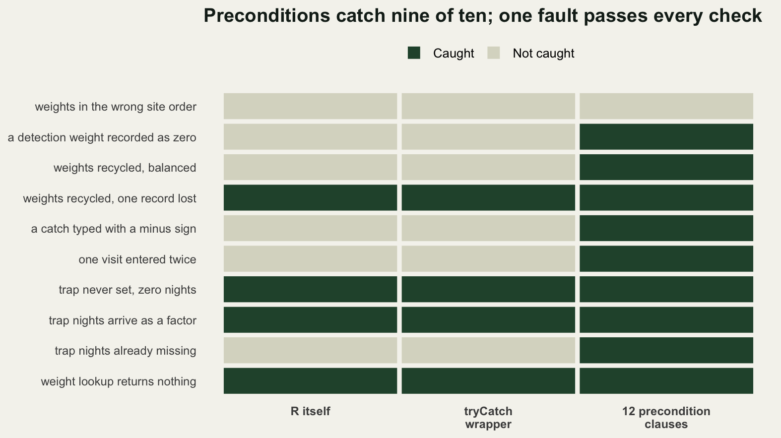
R speaks on 4 of the 10 faults. The other 6 pass in silence, and 5 of those 6 return a number that gets written down. The worst of the silent ones moves the reported effect by 23.3581 points, which is on the scale of the effect itself.
The tryCatch column is identical to the R column, and that is the point of putting it in the figure. A condition handler handles conditions. If nothing is signalled there is nothing to handle, so tryCatch around the whole analysis converts 2 errors and 2 warnings into 4 recorded messages and does not see the other 6 at all. It is the right tool for a different job: carrying on through a loop over a hundred sites when one of them fails, or attaching a better message to a failure you can predict. It is not a way of finding out whether the answer is right.
The 12 precondition clauses catch 9 of the 10, and the tryCatch wrapper costs 5 lines to duplicate what R already did. The guard is not free: check_inputs deparses to 9 lines against 10 for the analysis it protects, so the checking is very nearly as long as the thing checked. It is still cheap, because it is written once and then runs on every data set the function ever sees, and because every clause in it is a sentence an ecologist can read. Trap nights are a positive number. Catches are not negative. There is one weight per record. No site was visited twice on the same visit number. None of that is about programming, and all of it is a claim about how a pitfall trap survey works.
Two habits go with the guards. The first is to put them at the top of a function rather than in a script, so they travel with the code and run on every data set it ever sees; a check inside a script runs once, on the data that were in memory that afternoon. The second is that a guard is cheap only if it is specific: stopifnot(all(recs$nights > 0)) names the thing that failed, whereas a general assertion that the data are valid tells you nothing you did not already know.
For the moment when a guard does fire, R’s interactive tools are what you want next, and they are in this block rather than in a running chunk because they need a session with a person sitting at it:
# not run here: every one of these needs an interactive session
traceback()                 # the call stack of the error that just happened
options(error = recover)    # drop into a frame browser when anything errors
debug(analyse)              # step through the next call to analyse
undebug(analyse)
browser()                   # paste this into a function to stop at that line
options(warn = 2)           # turn every warning into an error, with a traceback
options(warn = 2) is the one worth knowing about for the recycling case, and it is also the one that explains why the recycling case is so bad. Turning warnings into errors would have caught the ragged version of the bug at once and would still have done nothing at all about the balanced one.
The honest limit
A precondition catches what it states. Nothing else. The tenth fault is the demonstration, and it is not an artificial one: the weight table is sorted by weight rather than by site code, and the analyst attaches it with rep(weight, each = 5) instead of matching on the code. That is a reasonable thing to type when the two tables started out in the same order.
bad_w <- rep(wt10$weight, each = n_visit)
bad_out <- observe(guarded(base_recs, bad_w))
bad_effect <- analyse(base_recs, bad_w)
bad_sm <- tapply(rate * bad_w, d$site, mean)

clause <- c(rows = nrow(base_recs) > 0,
            nights_numeric = is.numeric(base_recs$nights),
            catch_numeric = is.numeric(base_recs$catch),
            nights_finite = all(is.finite(base_recs$nights)),
            catch_finite = all(is.finite(base_recs$catch)),
            nights_positive = all(base_recs$nights > 0),
            catch_not_negative = all(base_recs$catch >= 0),
            weights_numeric = is.numeric(bad_w),
            one_weight_per_record = length(bad_w) == nrow(base_recs),
            weights_finite = all(is.finite(bad_w)),
            weights_in_range = all(bad_w > 0.4 & bad_w < 2.5),
            no_duplicate_visits = anyDuplicated(base_recs[, c("site", "visit")]) == 0)
print(clause)
rows nights_numeric catch_numeric
TRUE TRUE TRUE
nights_finite catch_finite nights_positive
TRUE TRUE TRUE
catch_not_negative weights_numeric one_weight_per_record
TRUE TRUE TRUE
weights_finite weights_in_range no_duplicate_visits
TRUE TRUE TRUE round(c(precondition_clauses = length(clause),
clauses_that_pass = sum(clause),
messages_from_the_guarded_run = length(bad_out$said),
weights_used = length(unique(bad_w)),
records_given_the_right_weight = sum(bad_w == base_w),
true_effect_percent = true_effect,
reported_effect_percent = bad_effect,
shift_in_points = bad_effect - true_effect,
pairs_reversed_percent = pair_flip(site_mean, bad_sm),
the_check_that_would_have_caught_it =
as.numeric(all(bad_w == as.numeric(w[base_recs$site])))), 4) precondition_clauses clauses_that_pass
12.0000 12.0000
messages_from_the_guarded_run weights_used
0.0000 12.0000
records_given_the_right_weight true_effect_percent
5.0000 22.5741
reported_effect_percent shift_in_points
-0.7840 -23.3581
pairs_reversed_percent the_check_that_would_have_caught_it
37.8788 0.0000 All 12 clauses pass. The guarded run produces 0 messages. The weight vector has one entry per record, all 12 distinct weights are present, every value is finite and inside the plausible range, and 5 of the 60 records happen to receive the weight they should. The reported grazing effect comes out at -0.7840 per cent against a true 22.5741, a shift of 23.3581 points, and on this run the sign does go. An analysis that should report a 22.6 per cent grazing effect reports none.
The check that would have caught it is in the last line of that chunk, and it is not a check about types or lengths. It compares the weight actually used against the weight the site code says it should be, which means it has to know what the join key is. That is the general shape of the limit: shape checks are cheap and catch a lot, and the errors they cannot see are the ones where the shape is right and the correspondence is wrong. Alignment between two tables is the commonest of those in ecology, because ecological data always arrive as several tables that have to be put next to each other, and the standard advice about it is worth repeating: never line tables up by position when a key exists, and check the result of the join rather than trusting it.
Two smaller limits belong here too. The precondition set was written after the ten faults were known, so 9 out of 10 is an optimistic figure in the same way that a test written after the bug is an optimistic test; the same argument appears in testing your analysis code, where the honest way to score a suite is to break the code on purpose. And every measurement in this post is one simulated survey with one seed. The mechanisms are exact and would repeat: as.numeric on a factor always returns the level index, and 60 always divides by 12. The sizes of the shifts are one draw from a distribution and would move if the survey were resampled.
Where to go next
The cheapest habit from this post is the smallest one: when you attach a vector to a table, check its length against the number of rows on the very next line, and when you read a column that should be a number, check that it is one. Reading field data into R is where those two checks belong, at the boundary between the spreadsheet and the analysis, and joining ecological tables without losing zeros is the post for the alignment problem that the last section could not solve.
Once the guards are in place they want to become assertions that run on their own. Testing your analysis code turns a precondition into a test with inputs chosen to break it, and checking an analysis script does the same thing one level up, asking whether the whole file runs from a clean session and reports the numbers it actually computed.
References
Wilson G, Bryan J, Cranston K, Kitzes J, Nederbragt L, Teal TK 2017 PLoS Computational Biology 13(6):e1005510 (10.1371/journal.pcbi.1005510)
Wilson G, Aruliah DA, Brown CT, Chue Hong NP, Davis M, Guy RT, Haddock SHD, Huff KD, Mitchell IM, Plumbley MD, Waugh B, White EP, Wilson P 2014 PLoS Biology 12(1):e1001745 (10.1371/journal.pbio.1001745)
Wickham H 2014 Journal of Statistical Software 59(10):1-23 (10.18637/jss.v059.i10)
Zuur AF, Ieno EN, Elphick CS 2010 Methods in Ecology and Evolution 1(1):3-14 (10.1111/j.2041-210X.2009.00001.x)
Ziemann M, Eren Y, El-Osta A 2016 Genome Biology 17:177 (10.1186/s13059-016-1044-7)
Chambers JM 2008 Software for Data Analysis: Programming with R, Springer (ISBN 978-0-387-75935-7)