library(ggplot2)

te_pal <- list(forest = "#275139", green = "#2f8f63", sage = "#93a87f",
               clay = "#b5534e", gold = "#cda23f", line = "#dad9ca",
               ink = "#16241d", paper = "#f5f4ee")

theme_te <- function() {
  theme_minimal(base_size = 12) +
    theme(panel.grid.minor = element_blank(),
          panel.grid.major = element_line(colour = "#e7e6dc"),
          plot.background = element_rect(fill = "#f5f4ee", colour = NA),
          panel.background = element_rect(fill = "#f5f4ee", colour = NA),
          plot.title = element_text(face = "bold", colour = te_pal$ink),
          axis.title = element_text(colour = "#2c3a31"))
}Git for ecologists
R
reproducibility
ecology tutorial
ggplot2
A twelve step editing history and eight manuscript figures: measure how many come back given the code state, the data version and the seed that produced them.
The manuscript went out in March. In September a reviewer asks for one of the figures to be redrawn with the patches ordered by area rather than by name, which is ten minutes of work. You open the project folder. There is a script, there is a data file, there are eight PNG files with the figure numbers in their names, and there is a subfolder called old containing five more scripts whose names all begin with analysis. You run the script. It works. The number it prints is not the number in the caption of the figure you were asked to redraw, and nothing in the folder tells you whether the difference is the script, the data file, or the fact that the figure was made on a Tuesday in April with a random subsample.
That is what version control is for. It is not backup: a backup gives you yesterday’s folder, and yesterday’s folder has the same problem. It is the answer to a question with a specific shape, “which state of the code produced this figure”, and the useful way to think about the answer is that it has three parts. The code state, the version of the data it read, and the state of the random number generator when it ran. A tool that records one of the three is not a third of the way there, because the parts do not add: this post measures exactly how far each combination gets you.
The measurement is a simulated woodland bird survey, twelve edits to the analysis script, and eight figures produced along the way. Everything is written in base R and nothing calls git, because the point is not the commands. The commands take an afternoon to learn and are printed near the end of the post. The point is what a commit has to contain before it answers the question, and how much your reported ecological result moves when it does not.
The survey, and three versions of the data file
Twenty four woodland patches spread over a bit more than two orders of magnitude of area, thirty bird species counted at point counts in each patch. Twelve of the species occur anywhere. The other eighteen have an area threshold below which they are absent, spread from a hectare up to ninety, so that a larger patch holds both more individuals and a larger species pool. That is a species area relationship built by hand, and the quantity the manuscript reports is its slope: how many species are added per tenfold increase in patch area.
set.seed(20260817)

n_patch <- 24
n_spec  <- 30
patch <- sprintf("P%02d", seq_len(n_patch))
area  <- round(exp(seq(log(0.8), log(160), length.out = n_patch)) *
                 exp(rnorm(n_patch, 0, 0.12)), 2)
guild <- rep(c("ground", "canopy", "aerial"), length.out = n_spec)

a_s <- rnorm(n_spec, 1.35, 0.4)
b_s <- rnorm(n_spec, 0.05, 0.12)
thr <- c(rep(0, 12), round(exp(seq(log(1.2), log(90), length.out = n_spec - 12)), 2))
lam <- exp(outer(rep(1, n_patch), a_s) + outer(log10(area), b_s)) * outer(area, thr, ">=")
cnt <- matrix(rpois(n_patch * n_spec, lam), n_patch, n_spec)

d2 <- data.frame(patch = rep(patch, times = n_spec),
                 area = rep(area, times = n_spec),
                 species = rep(sprintf("sp%02d", seq_len(n_spec)), each = n_patch),
                 guild = rep(guild, each = n_patch),
                 count = as.vector(cnt), stringsAsFactors = FALSE)
d2 <- d2[order(d2$patch, d2$species), ]
rownames(d2) <- NULL

round(c(patches = n_patch, species = n_spec,
        smallest_patch_hectares = min(area), largest_patch_hectares = max(area),
        species_with_no_area_threshold = sum(thr == 0),
        individuals = sum(d2$count),
        smallest_patch_individuals = min(tapply(d2$count, d2$patch, sum)),
        largest_patch_individuals = max(tapply(d2$count, d2$patch, sum))), 4)
patches species
24.00 30.00
smallest_patch_hectares largest_patch_hectares
0.73 167.44
species_with_no_area_threshold individuals
12.00 2425.00
smallest_patch_individuals largest_patch_individuals
41.00 170.00 print(head(d2, 4)) patch area species guild count
1 P01 0.73 sp01 ground 2
2 P01 0.73 sp02 canopy 6
3 P01 0.73 sp03 aerial 6
4 P01 0.73 sp04 ground 2The data file has a history of its own, which is the part most projects forget. The first export carries four counts entered with a trailing zero and two records that were pasted in twice when the two field notebooks were merged. That is version one. A data check catches those and produces version two. In August the late season visits are added for seven patches, which is version three. All three versions have lived in the folder under the same file name at different times, which is the ordinary way for a data file to change.
d1 <- d2
err_rows <- c(37, 210, 388, 501)
d1$count[err_rows] <- d1$count[err_rows] * 10L
d1 <- rbind(d1, d2[c(96, 415), ])
d1 <- d1[order(d1$patch, d1$species), ]
rownames(d1) <- NULL

set.seed(20260818)
d3 <- d2
sel <- d3$patch %in% patch[c(2, 5, 9, 13, 18, 21, 24)]
d3$count[sel] <- d3$count[sel] + rpois(sum(sel), 0.55)

datasets <- list(d1 = d1, d2 = d2, d3 = d3)
round(rbind(rows = sapply(datasets, nrow),
            individuals = sapply(datasets, function(z) sum(z$count)),
            largest_count = sapply(datasets, function(z) max(z$count))), 4)
d1 d2 d3
rows 722 720 720
individuals 2544 2425 2541
largest_count 70 16 16round(c(records_altered = length(err_rows), records_pasted_twice = 2,
inflation_in_version_one_percent = 100 * (sum(d1$count) / sum(d2$count) - 1),
added_by_the_late_visits_percent = 100 * (sum(d3$count) / sum(d2$count) - 1)), 4) records_altered records_pasted_twice
4.0000 2.0000
inflation_in_version_one_percent added_by_the_late_visits_percent
4.9072 4.7835 Version one carries 722 rows against the 720 of the checked file, and 2544 individuals against 2425, an inflation of the total catch by 4.9072 per cent sitting in six records. Version three adds the late visits and comes to 2541 individuals, 4.7835 per cent above version two. None of the three announces itself. A file called patch_counts.csv looks the same on every one of those days.
The script, and twelve edits to it
The analysis is one function. It sums the catch per patch, counts the species, and regresses richness on the base ten logarithm of patch area. The function is held here as a character vector of lines so that edits to it can be made, compared and compiled the way a version control system sees them: as text.
v0 <- c(
"report_slope <- function(dat) {",
"  d <- dat",
"  eff <- tapply(d$count, d$patch, sum)",
"  patches <- names(eff)",
"  rich <- sapply(patches, function(p) sum(d$count[d$patch == p] > 0))",
"  area <- sapply(patches, function(p) d$area[d$patch == p][1])",
"  fit <- lm(rich ~ log10(area))",
"  unname(coef(fit)[2])",
"}")

compile <- function(src) {
  e <- new.env(parent = globalenv())
  eval(parse(text = paste(src, collapse = "\n")), envir = e)
  get("report_slope", envir = e)
}
c(lines_in_the_first_version = length(v0))
lines_in_the_first_version
9 round(c(first_reported_gradient = compile(v0)(d1)), 4)first_reported_gradient
8.5531 Now the edits. Twelve of them, in the order an analysis really grows. Seven move the reported number: a rule that drops the species seen once, a filter that seemed sensible after looking at the effort column, a decision to rarefy rather than to count species raw, a change of mind about the rarefaction depth, a guild that the co-author wanted excluded, a second thought about where the effort threshold should sit, and a patch that turned out to have been flooded. The other five touch only the text. Each edit is written as a transformation of the line vector, so that the versions are genuinely derived from one another rather than typed out separately.
repl <- function(x, from, to) { i <- which(x == from); x[i] <- to; x }
ins_after <- function(x, from, new) append(x, new, after = which(x == from))
del <- function(x, from) x[-which(x == from)]

edits <- list(
  list(lab = "singletons dropped", kind = "consequential",
       f = function(x)
         repl(x, "  rich <- sapply(patches, function(p) sum(d$count[d$patch == p] > 0))",
              "  rich <- sapply(patches, function(p) sum(d$count[d$patch == p] > 1))")),
  list(lab = "comment added", kind = "cosmetic",
       f = function(x) ins_after(x, "report_slope <- function(dat) {",
                                 "  # dat: one row per patch and species")),
  list(lab = "effort filter", kind = "consequential",
       f = function(x) ins_after(x, "  eff <- tapply(d$count, d$patch, sum)",
                                 c("  ok <- names(eff)[eff >= 45]",
                                   "  d <- d[d$patch %in% ok, ]",
                                   "  eff <- eff[ok]"))),
  list(lab = "rarefaction", kind = "consequential",
       f = function(x) {
         x <- repl(x, "report_slope <- function(dat) {",
                   "report_slope <- function(dat, depth = 30) {")
         repl(x, "  rich <- sapply(patches, function(p) sum(d$count[d$patch == p] > 1))",
              paste("  rich <- sapply(patches, function(p) length(unique(sample(rep(",
                    "d$species[d$patch == p], d$count[d$patch == p]), depth))))"))
       }),
  list(lab = "two lines reordered", kind = "cosmetic",
       f = function(x) {
         ln <- "  area <- sapply(patches, function(p) d$area[d$patch == p][1])"
         ins_after(del(x, ln), "  patches <- names(eff)", ln)
       }),
  list(lab = "depth 30 to 40", kind = "consequential",
       f = function(x) repl(x, "report_slope <- function(dat, depth = 30) {",
                            "report_slope <- function(dat, depth = 40) {")),
  list(lab = "aerial guild dropped", kind = "consequential",
       f = function(x) ins_after(x, "  d <- dat", '  d <- d[d$guild != "aerial", ]')),
  list(lab = "comment reworded", kind = "cosmetic",
       f = function(x) repl(x, "  # dat: one row per patch and species",
                            "  # dat: one row per patch and species, counts as integers")),
  list(lab = "filter 45 to 60", kind = "consequential",
       f = function(x) repl(x, "  ok <- names(eff)[eff >= 45]",
                            "  ok <- names(eff)[eff >= 60]")),
  list(lab = "variable renamed", kind = "cosmetic",
       f = function(x) gsub("\\bd\\$", "sur$",
                            gsub("(^|[^$._[:alnum:]])d($|[^$._[:alnum:]])", "\\1sur\\2", x))),
  list(lab = "flooded patch dropped", kind = "consequential",
       f = function(x) ins_after(x, "  sur <- dat", '  sur <- sur[sur$patch != "P17", ]')),
  list(lab = "header comment", kind = "cosmetic",
       f = function(x) c("# slope of rarefied richness on log10 patch area",
                         "# figure 2 of the manuscript", x)))

code <- vector("list", length(edits) + 1)
code[[1]] <- v0
for (k in seq_along(edits)) code[[k + 1]] <- edits[[k]]$f(code[[k]])
fun <- lapply(code, compile)
state_of <- function(v, dv, seed) { set.seed(seed); fun[[v + 1]](datasets[[dv]]) }

kinds <- sapply(edits, `[[`, "kind")
c(edits = length(edits), code_states = length(code),
  consequential_by_intent = sum(kinds == "consequential"),
  cosmetic_by_intent = sum(kinds == "cosmetic"),
  lines_in_the_last_version = length(code[[13]]))
edits code_states consequential_by_intent
12 13 7
cosmetic_by_intent lines_in_the_last_version
5 17 cat(code[[13]], sep = "\n")# slope of rarefied richness on log10 patch area
# figure 2 of the manuscript
report_slope <- function(dat, depth = 40) {
# dat: one row per patch and species, counts as integers
sur <- dat
sur <- sur[sur$patch != "P17", ]
sur <- sur[sur$guild != "aerial", ]
eff <- tapply(sur$count, sur$patch, sum)
ok <- names(eff)[eff >= 60]
sur <- sur[sur$patch %in% ok, ]
eff <- eff[ok]
patches <- names(eff)
area <- sapply(patches, function(p) sur$area[sur$patch == p][1])
rich <- sapply(patches, function(p) length(unique(sample(rep( sur$species[sur$patch == p], sur$count[sur$patch == p]), depth))))
fit <- lm(rich ~ log10(area))
unname(coef(fit)[2])
}The last version is the one on your disk today. It rarefies every patch to forty individuals, excludes patches with fewer than sixty individuals of the two remaining guilds, drops the flooded patch, and reports the slope of rarefied richness on log area. Nothing about it says what it used to be. Run all thirteen states against the current data file and the current seed and the history becomes visible.
sl <- sapply(0:12, function(v) state_of(v, "d3", 202))
names(sl) <- paste0("v", 0:12)
print(round(sl, 4))
v0 v1 v2 v3 v4 v5 v6 v7 v8 v9 v10
7.5303 7.3117 7.3117 7.2227 2.6793 2.6793 3.8529 2.9547 2.9547 2.2390 2.2390
v11 v12
3.1549 3.1549 round(c(distinct_answers = length(unique(round(sl, 8))),
states = length(sl),
lowest = min(sl), highest = max(sl),
spread = diff(range(sl)),
first_state = sl[["v0"]], last_state = sl[["v12"]]), 4)distinct_answers states lowest highest
8.0000 13.0000 2.2390 7.5303
spread first_state last_state
5.2914 7.5303 3.1549 Thirteen states of the script give 8 distinct answers, from 2.239 to 7.5303 species per tenfold increase in area. The five states that repeat a value are the five text-only edits, and that is worth holding on to: an edit either moves the number or it does not, and the file gives no sign of which kind it was.
Eight of those states produced a figure. The provenance table below is the one thing in this post that a real project does not have: it records, for each figure in the manuscript, which state of the code drew it, which version of the data file it read, and what the seed was. Figures one to three came from states with no random step in them, so their seed is irrelevant. Figures four, five, seven and eight were drawn by a script that seeded its resampling, and the seed was written down at the time, so it is recoverable; but it was written beside the figure rather than into the script, and none of the thirteen code states carries a trace of it. Figure six was drawn after the analyst pasted a corrected line into the console and re-ran the middle of the script, so its seed is whatever the generator happened to hold at that moment: a real number, never written anywhere.
figs <- data.frame(fig = 1:8,
                   code = c(0, 1, 3, 4, 6, 7, 9, 11),
                   data = c("d1", "d1", "d1", "d2", "d2", "d2", "d3", "d3"),
                   seed = c(NA, NA, NA, 101, 101, NA, 202, 202),
                   stringsAsFactors = FALSE)
lost_seed <- 4871
true_seed <- ifelse(is.na(figs$seed), c(777, 777, 777, 0, 0, lost_seed, 0, 0), figs$seed)
now <- list(code = 12, data = "d3", seed = 202)

figs$value <- sapply(1:8, function(i) state_of(figs$code[i], figs$data[i], true_seed[i]))
figs$stochastic <- figs$code >= 4
print(figs)
fig code data seed value stochastic
1 1 0 d1 NA 8.553139 FALSE
2 2 1 d1 NA 7.808002 FALSE
3 3 3 d1 NA 7.872166 FALSE
4 4 4 d2 101 2.731310 TRUE
5 5 6 d2 101 4.202769 TRUE
6 6 7 d2 NA 3.695214 TRUE
7 7 9 d3 202 2.238962 TRUE
8 8 11 d3 202 3.154943 TRUEround(c(figures = nrow(figs),
distinct_code_states = length(unique(figs$code)),
deterministic_figures = sum(!figs$stochastic),
figures_with_a_recorded_seed = sum(!is.na(figs$seed)),
lowest_reported = min(figs$value), highest_reported = max(figs$value)), 4) figures distinct_code_states
8.0000 8.0000
deterministic_figures figures_with_a_recorded_seed
3.0000 4.0000
lowest_reported highest_reported
2.2390 8.5531 The eight captions in the manuscript therefore claim gradients from 2.239 to 8.5531 species per tenfold increase in area, which is a factor of nearly four across figures that all describe the same survey. Every one of them was correct on the day it was made.
Which of the eight come back
Here is the measurement the post exists for. Take each figure in turn and try to rebuild the number in its caption. You are allowed to know some subset of three things: the code state, the data version, and the seed. Whatever you are not told, you supply from what is in the folder today, which is the last version of the script, the current data file, and the seed written at the top of that script. A figure counts as reconstructed when the rebuilt number equals the recorded one exactly.
recon <- function(i, kc, kd, ks) {
  v  <- if (kc) figs$code[i] else now$code
  dv <- if (kd) figs$data[i] else now$data
  s  <- if (ks && !is.na(figs$seed[i])) figs$seed[i] else now$seed
  state_of(v, dv, s)
}
same <- function(a, b) isTRUE(all.equal(a, b, tolerance = 1e-10))

grid <- expand.grid(code = c(FALSE, TRUE), data = c(FALSE, TRUE), seed = c(FALSE, TRUE))
grid$known <- apply(grid[, 1:3], 1, function(z)
  if (!any(z)) "nothing" else paste(c("code", "data", "seed")[z], collapse = " + "))
grid$hits <- sapply(seq_len(nrow(grid)), function(g)
  sum(sapply(1:8, function(i)
    same(recon(i, grid$code[g], grid$data[g], grid$seed[g]), figs$value[i]))))
grid$worst <- sapply(seq_len(nrow(grid)), function(g)
  max(abs(sapply(1:8, function(i)
    recon(i, grid$code[g], grid$data[g], grid$seed[g])) - figs$value)))
print(grid[order(grid$hits), c("known", "hits", "worst")], digits = 5)
known hits worst
1 nothing 1 5.39820
3 data 1 4.58379
5 seed 1 5.39820
7 data + seed 1 4.58379
2 code 2 1.02283
6 code + seed 2 1.02283
4 code + data 5 0.72668
8 code + data + seed 7 0.23015round(c(nothing_known = grid$hits[grid$known == "nothing"],
code_only = grid$hits[grid$known == "code"],
data_only = grid$hits[grid$known == "data"],
seed_only = grid$hits[grid$known == "seed"],
code_and_data = grid$hits[grid$known == "code + data"],
seed_and_data = grid$hits[grid$known == "data + seed"],
all_three = grid$hits[grid$known == "code + data + seed"],
worst_error_with_nothing = max(grid$worst),
worst_error_with_code_and_data = grid$worst[grid$known == "code + data"],
worst_error_with_all_three = grid$worst[grid$known == "code + data + seed"]), 4) nothing_known code_only
1.0000 2.0000
data_only seed_only
1.0000 1.0000
code_and_data seed_and_data
5.0000 1.0000
all_three worst_error_with_nothing
7.0000 5.3982
worst_error_with_code_and_data worst_error_with_all_three
0.7267 0.2301 The test is exact equality, to every digit R holds, and that is deliberate. A looser test would let a figure count as reconstructed when the rebuilt number happens to round the same way at the two decimals a caption prints, which is a statement about the printing rather than about the analysis. It would also be unstable in the direction that flatters the tool: the coarser the printed value, the more reconstructible the figure looks. If the rebuilt number is not the recorded number, the figure came from something other than what you ran, and the useful question is what.
comp <- grid[order(grid$hits, grid$known), ]
comp$known <- factor(comp$known, levels = comp$known)

ggplot(comp, aes(hits, known)) +
  geom_col(fill = te_pal$forest, width = 0.66) +
  geom_text(aes(label = hits), hjust = -0.5, colour = te_pal$ink, size = 3.8) +
  scale_x_continuous(limits = c(0, 8.6), breaks = 0:8) +
  labs(x = "Figures rebuilt exactly, out of eight", y = "What you know",
       title = "No two of the three components rebuild more than five figures") +
  theme_te()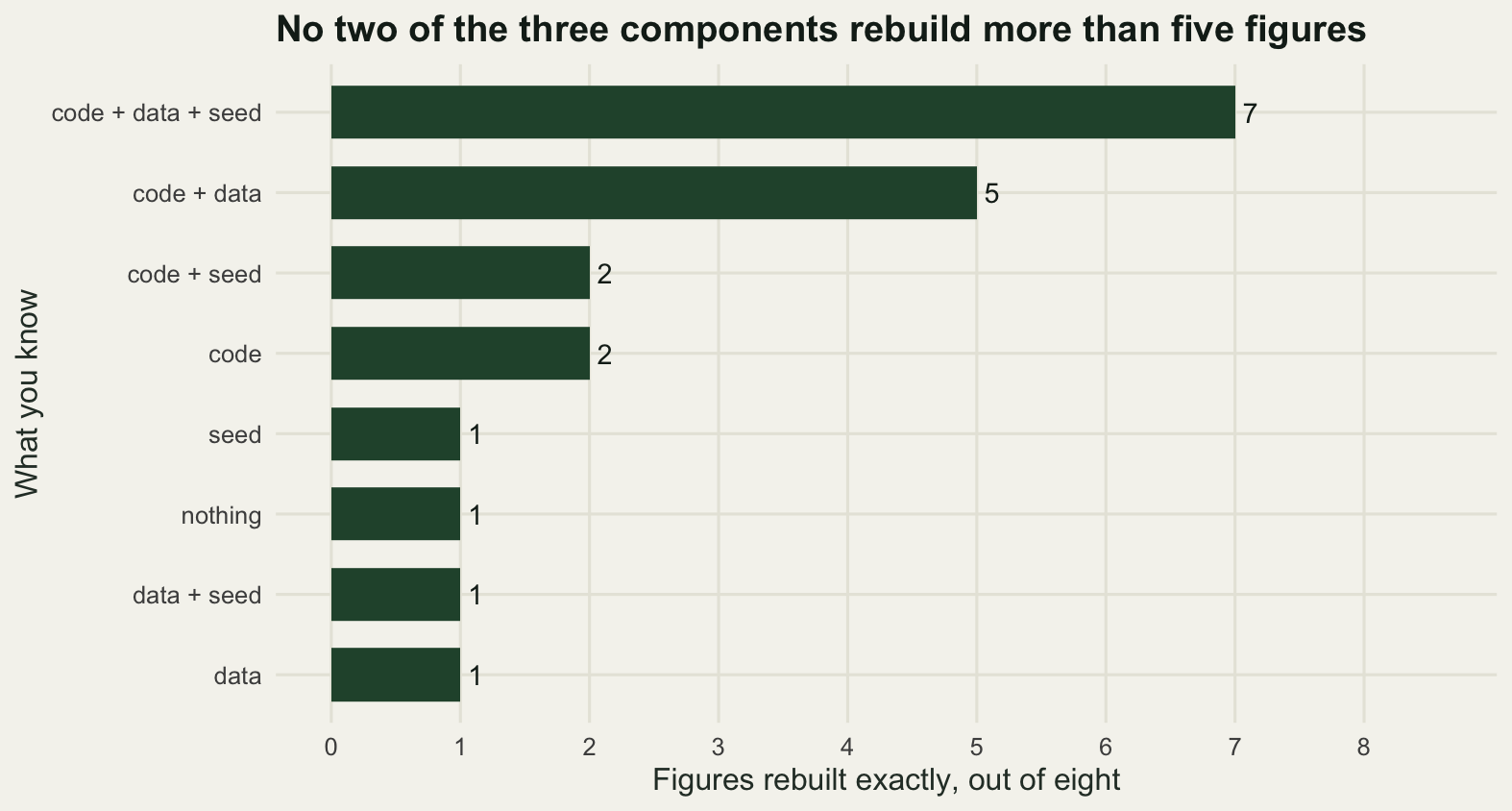
Knowing nothing beyond what is in the folder rebuilds 1 of the 8 figures. That one is the last figure drawn, and it survives only because the twelfth edit was a comment: the state that drew it and the state on disk are different files that compute the same number.
Knowing the code state, which is what a perfect commit history gives you and nothing else, rebuilds 2 of 8. That is the number to take away from this section. Version control of the script, done properly, with a commit for every edit and a tag on the commit that drew each figure, answers a quarter of the question. The other figures fail because they read a data file that has since been replaced, or because they were seeded differently, and no amount of discipline about the script touches either.
Code and data together rebuild 5 of 8. All three rebuild 7. The eighth is figure six, and it cannot be rebuilt by anybody, ever, because its seed was never written down. The closest approach leaves 0.2301 species per tenfold area between the rebuilt value and the one in the caption, which is a small error and is still an error, and the honest description of that figure is that its caption cannot be checked.
today <- sapply(1:8, function(i) recon(i, FALSE, FALSE, FALSE))
gap <- 100 * (today - figs$value) / figs$value
print(round(rbind(recorded = figs$value, from_todays_folder = today, difference_percent = gap), 4))
[,1] [,2] [,3] [,4] [,5] [,6] [,7]
recorded 8.5531 7.8080 7.8722 2.7313 4.2028 3.6952 2.2390
from_todays_folder 3.1549 3.1549 3.1549 3.1549 3.1549 3.1549 3.1549
difference_percent -63.1136 -59.5935 -59.9228 15.5102 -24.9318 -14.6208 40.9109
[,8]
recorded 3.1549
from_todays_folder 3.1549
difference_percent 0.0000round(c(figures_matching_today = sum(abs(gap) < 1e-8),
largest_overstatement_percent = max(gap),
largest_understatement_percent = min(gap),
mean_absolute_gap_percent = mean(abs(gap)),
largest_absolute_gap_species = max(abs(today - figs$value))), 4) figures_matching_today largest_overstatement_percent
1.0000 40.9109
largest_understatement_percent mean_absolute_gap_percent
-63.1136 34.8255
largest_absolute_gap_species
5.3982 dr <- data.frame(fig = factor(rep(sprintf("Figure %d", 1:8), 2),
levels = rev(sprintf("Figure %d", 1:8))),
value = c(figs$value, today),
source = factor(rep(c("Recorded in the caption",
"Rebuilt from today's folder"), each = 8),
levels = c("Recorded in the caption",
"Rebuilt from today's folder")))
seg <- data.frame(fig = factor(sprintf("Figure %d", 1:8),
levels = rev(sprintf("Figure %d", 1:8))),
lo = pmin(figs$value, today), hi = pmax(figs$value, today))
ggplot(dr, aes(value, fig)) +
geom_segment(data = seg, aes(x = lo, xend = hi, y = fig, yend = fig),
inherit.aes = FALSE, colour = te_pal$line, linewidth = 1.6) +
geom_point(aes(shape = source, colour = source), size = 3.4, stroke = 1.1) +
scale_shape_manual(values = c(1, 16), name = NULL) +
scale_colour_manual(values = c(te_pal$forest, te_pal$clay), name = NULL) +
scale_x_continuous(limits = c(0, 9.2)) +
labs(x = "Reported gradient (species per tenfold increase in area)", y = NULL,
title = "Eight captions, one folder, and one number it can still produce") +
theme_te() +
theme(legend.position = "top")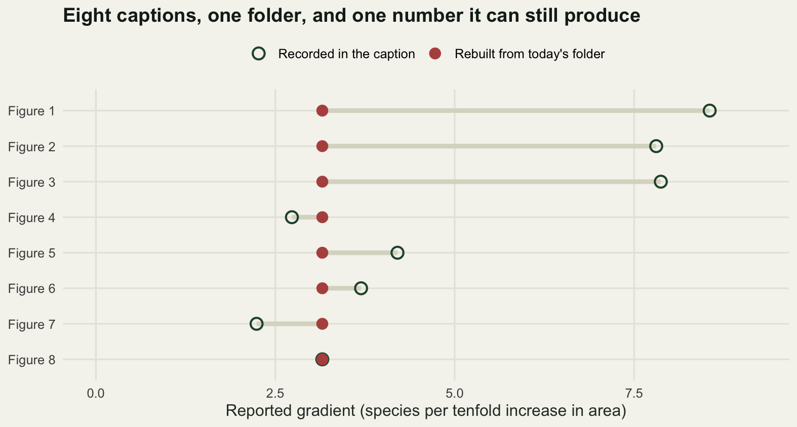
Across the eight figures the rebuilt value is out by 34.8255 per cent on average. The worst case is the first figure, which reported 8.5531 and now comes back as 3.1549, an understatement of 63.1136 per cent, and the largest absolute gap is 5.3982 species per tenfold increase in area. Two of the gaps go the other way: figures four and seven are now overstated, by 15.5102 and 40.9109 per cent. The direction is not a property of time, it is a property of which edits happened to sit between the figure and today.
One thing that measurement hides is that the three components are not the same size. The code and the data move the answer by a lot; the seed moves it by a little. Two hundred seeds, with the code and data held at each figure’s own values, put a number on the little.
set.seed(5)
seeds <- sample(1e5, 200)
noise <- sapply(4:8, function(i) {
  z <- sapply(seeds, function(s) { set.seed(s); fun[[figs$code[i] + 1]](datasets[[figs$data[i]]]) })
  c(sd = sd(z), range = diff(range(z)), rel = 100 * sd(z) / abs(figs$value[i]))
})
colnames(noise) <- sprintf("fig%d", 4:8)
print(round(noise, 4))
fig4 fig5 fig6 fig7 fig8
sd 0.4822 0.4552 0.3885 0.6298 0.6586
range 2.4572 2.4404 2.0723 3.4193 3.6783
rel 17.6560 10.8313 10.5148 28.1292 20.8757round(c(seeds = length(seeds),
mean_sd_across_seeds = mean(noise["sd", ]),
largest_range_across_seeds = max(noise["range", ]),
largest_relative_sd_percent = max(noise["rel", ]),
worst_seed_only_error = grid$worst[grid$known == "code + data"]), 4) seeds mean_sd_across_seeds
200.0000 0.5229
largest_range_across_seeds largest_relative_sd_percent
3.6783 28.1292
worst_seed_only_error
0.7267 The seed is the smallest of the three components and it is not negligible. Holding the code and the data at the values that drew each figure and changing only the seed moves the gradient with a standard deviation of 0.5229 species per tenfold area, up to 3.6783 between the extreme seeds, and the largest failed reconstruction in the code and data row of the table above is out by 0.7267. On a figure reporting 2.7313, a standard deviation of 0.4822 is 17.656 per cent of the estimate. Anybody quoting that gradient to four decimal places is quoting three digits of a random number generator.
One thing worth trying before giving up on a folder is the search. If you happen to hold every state of the script, every version of the data file and a short list of plausible seeds, you can run all the combinations and ask which of them reproduces each caption. That is not a realistic position to be in, because it assumes the history this post is about, but it puts an upper bound on what archaeology can do.
cand <- expand.grid(state = 0:12, data = names(datasets), seed = c(101, 202, 777),
                    stringsAsFactors = FALSE)
cand$value <- mapply(state_of, cand$state, cand$data, cand$seed)

hit <- lapply(figs$value, function(v) cand[abs(cand$value - v) < 1e-10, ])
found <- data.frame(fig = 1:8,
                    combinations = sapply(hit, nrow),
                    states = sapply(hit, function(h) length(unique(h$state))),
                    data_versions = sapply(hit, function(h) length(unique(h$data))),
                    true_state = figs$code, stringsAsFactors = FALSE)
print(found, row.names = FALSE)
fig combinations states data_versions true_state
1 3 1 1 0
2 6 2 1 1
3 3 1 1 3
4 2 2 1 4
5 1 1 1 6
6 0 0 0 7
7 2 2 1 9
8 2 2 1 11round(c(combinations_searched = nrow(cand),
figures_matched = sum(found$states > 0),
figures_unmatched = sum(found$states == 0),
pinned_to_one_state = sum(found$states == 1),
ambiguous_between_two_states = sum(found$states == 2),
data_version_always_unambiguous = all(found$data_versions[found$states > 0] == 1),
true_state_among_the_matches =
sum(sapply(1:8, function(i) figs$code[i] %in% hit[[i]]$state))), 4) combinations_searched figures_matched
117 7
figures_unmatched pinned_to_one_state
1 3
ambiguous_between_two_states data_version_always_unambiguous
4 1
true_state_among_the_matches
7 The search runs 117 combinations, matches 7 of the 8 figures, and in every one of those 7 the state that really drew the figure is among the matches. Figure six is the one it misses, for the reason it has been missing all along. Of the seven it matches, only 3 are pinned to a single state of the script: the other 4 are matched equally well by two adjacent states, because a cosmetic edit sits between them and the two states are different files that compute the same number. The data version comes out unambiguous every time, which is a fact about this history rather than a general one: three data versions that differ by a few dozen counts are easy to tell apart, and two that differ in one cell would not be.
So the upper bound on archaeology is that it recovers the equivalence class of the code, not the code. If the question is which number the figure showed, the search answers it. If the question is which file to edit so that the reviewer’s version matches the original, a class of two states is still a guess.
The analysis_final_v3_REAL.R pattern
Nobody arrives at that folder through carelessness. They arrive through a version control system that everybody invents independently, which is to save a copy under a new name whenever the changes feel large enough to be worth keeping. It is a real system, it costs nothing to learn, and it can be scored the same way as any other. Here is the naming history that goes with the twelve edits above: three states saved over one another as analysis.R, three as analysis_v2.R, and so on, with one copy taken as a backup on the day the co-author’s comments arrived.
saves <- data.frame(
  state = c(0:12, 7),
  file = c(rep("analysis.R", 3), rep("analysis_v2.R", 3), rep("analysis_final.R", 2),
           rep("analysis_final_v2.R", 2), rep("analysis_final_v3_REAL.R", 3),
           "analysis_final_backup.R"),
  stringsAsFactors = FALSE)
saves <- saves[order(saves$state), ]

txt_of <- sapply(code, function(z) paste(z, collapse = "\n"))
disk <- tapply(saves$state, saves$file, max)
kept <- sort(unique(as.integer(disk)))
print(disk)
analysis_final_backup.R analysis_final_v2.R analysis_final_v3_REAL.R
7 9 12
analysis_final.R analysis_v2.R analysis.R
7 5 2 round(c(saves = nrow(saves),
file_names = length(disk),
states_in_the_history = length(code),
states_still_readable = length(kept),
states_destroyed_by_overwriting = length(code) - length(kept),
identical_content_under_two_names = sum(duplicated(txt_of[as.integer(disk) + 1])),
figure_states_still_readable = sum(figs$code %in% kept),
figure_states_lost = sum(!figs$code %in% kept),
distinct_answers_still_readable = length(unique(round(sl[kept + 1], 8))),
distinct_answers_in_the_history = length(unique(round(sl, 8)))), 4) saves file_names
14 6
states_in_the_history states_still_readable
13 5
states_destroyed_by_overwriting identical_content_under_two_names
8 1
figure_states_still_readable figure_states_lost
2 6
distinct_answers_still_readable distinct_answers_in_the_history
5 8 print(data.frame(file = names(disk), holds_state = as.integer(disk),
gradient = round(sl[as.integer(disk) + 1], 4)), row.names = FALSE) file holds_state gradient
analysis_final_backup.R 7 2.9547
analysis_final_v2.R 9 2.2390
analysis_final_v3_REAL.R 12 3.1549
analysis_final.R 7 2.9547
analysis_v2.R 5 2.6793
analysis.R 2 7.3117rows <- c("git: one commit per edit",
names(sort(tapply(saves$state, saves$file, min))))
nm <- data.frame(state = c(0:12, saves$state),
row = factor(c(rep(rows[1], 13), saves$file), levels = rev(rows)),
kept = c(rep(TRUE, 13),
saves$state == disk[match(saves$file, names(disk))]))
nm$kept <- factor(ifelse(nm$kept, "still readable at the end", "overwritten"),
levels = c("still readable at the end", "overwritten"))
band <- data.frame(lo = figs$code - 0.32, hi = figs$code + 0.32)
held <- txt_of[as.integer(disk) + 1]
twins <- names(disk)[held %in% held[duplicated(held)]]
tx <- max(disk[twins])
ggplot(nm, aes(state, row)) +
geom_rect(data = band, aes(xmin = lo, xmax = hi, ymin = -Inf, ymax = Inf),
inherit.aes = FALSE, fill = te_pal$line, alpha = 0.55) +
annotate("segment", x = tx + 0.42, xend = tx + 0.42, y = twins[1], yend = twins[2],
colour = te_pal$ink, linewidth = 0.45) +
annotate("segment", x = tx + 0.32, xend = tx + 0.42, y = twins, yend = twins,
colour = te_pal$ink, linewidth = 0.45) +
annotate("text", x = tx + 0.6, y = twins[2], hjust = 0, vjust = -0.3, size = 3.1,
colour = te_pal$ink, label = "identical text, two names") +
geom_point(aes(fill = kept), shape = 21, size = 3.6, colour = te_pal$ink, stroke = 0.7) +
scale_fill_manual(values = c(te_pal$forest, te_pal$paper), name = NULL) +
scale_x_continuous(breaks = 0:12) +
labs(x = "State of the script, from the first version to the twelfth edit", y = NULL,
title = "Saving under a new name keeps five of the thirteen states") +
theme_te() +
theme(legend.position = "top", panel.grid.major.y = element_blank())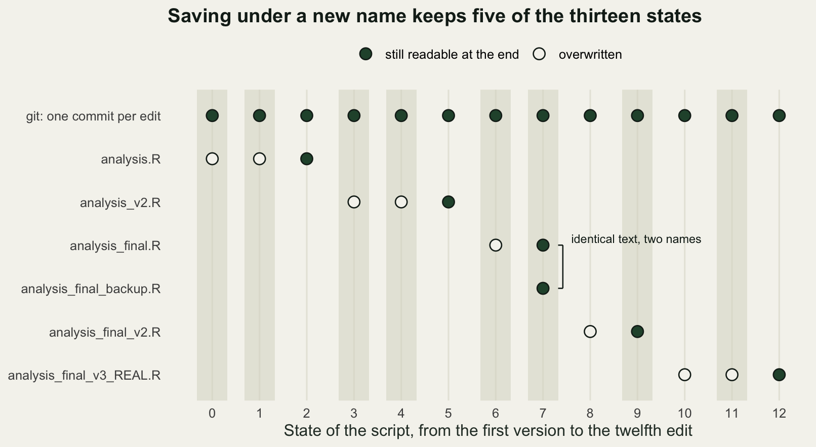
Fourteen saves produce 6 file names and leave 5 of the 13 states readable. The other 8 were overwritten by a later save under the same name, and they are gone in the strong sense: no copy exists anywhere. Of the eight states that drew a figure, 2 survive. Which two survive is an accident of where the saves happened to fall rather than a property of the scheme, and a commit for every edit would have left all eight readable.
Two smaller failures are visible in the same table. analysis_final.R and analysis_final_backup.R hold identical text: 1 pair of files that cannot be told apart by content, only by the story behind the names. And of the 8 distinct answers the history contains, the five surviving states carry 5, so three of the answers this script was capable of giving cannot be recomputed from any file in the folder even by somebody who knows which file to run.
The deeper problem is not the arithmetic. It is that a file name is a claim about which version is current, made by a person, at a moment when they were thinking about something else. analysis.R holds the second state, analysis_final_v3_REAL.R holds the twelfth, and nothing but the names suggests the order. A commit history makes the same claim mechanically, in the order the work happened, and it does not need anybody to be careful on a Friday afternoon.
A diff in twenty eight lines of base R
The other half of version control is the comparison. git diff shows you which lines changed between two states, and it is worth writing one, because the thing that makes a diff useful is also the thing that makes it misleading. A diff is a statement about text. The question you are asking is about numbers.
The standard algorithm finds the longest common subsequence of the two line vectors and reports everything outside it. The table is filled from the bottom right so that L[i, j] holds the length of the longest common subsequence of the two tails, and the walk from the top left then takes the matching line when it can and otherwise removes or adds whichever side keeps the most in common.
line_diff <- function(a, b) {
  n <- length(a); m <- length(b)
  L <- matrix(0L, n + 1, m + 1)
  for (i in n:1) for (j in m:1)
    L[i, j] <- if (a[i] == b[j]) L[i + 1, j + 1] + 1L else max(L[i + 1, j], L[i, j + 1])
  i <- 1; j <- 1; out <- character(0)
  while (i <= n && j <= m) {
    if (a[i] == b[j]) { i <- i + 1; j <- j + 1 }
    else if (L[i + 1, j] >= L[i, j + 1]) { out <- c(out, paste("-", a[i])); i <- i + 1 }
    else { out <- c(out, paste("+", b[j])); j <- j + 1 }
  }
  c(out, if (i <= n) paste("-", a[i:n]), if (j <= m) paste("+", b[j:m]))
}
c(lines_of_diff_code = length(deparse(line_diff)),
  lines_in_the_ninth_edit_diff = length(line_diff(code[[9]], code[[10]])),
  lines_between_the_two_surviving_files = length(line_diff(code[[3]], code[[10]])))
lines_of_diff_code lines_in_the_ninth_edit_diff
28 2
lines_between_the_two_surviving_files
10 cat(line_diff(code[[9]], code[[10]]), sep = "\n")- ok <- names(eff)[eff >= 45]
+ ok <- names(eff)[eff >= 60]cat("\n")cat(line_diff(code[[3]], code[[10]]), sep = "\n")- report_slope <- function(dat) {
- # dat: one row per patch and species
+ report_slope <- function(dat, depth = 40) {
+ # dat: one row per patch and species, counts as integers
+ d <- d[d$guild != "aerial", ]
+ ok <- names(eff)[eff >= 60]
+ d <- d[d$patch %in% ok, ]
+ eff <- eff[ok]
- rich <- sapply(patches, function(p) sum(d$count[d$patch == p] > 1))
+ rich <- sapply(patches, function(p) length(unique(sample(rep( d$species[d$patch == p], d$count[d$patch == p]), depth))))The comparator comes to 28 lines as R deparses it, which is the way every other piece of machinery in this cluster of posts is counted. The first of the two diffs it prints is the ninth edit, and it is the whole of that edit: one comparison moves from forty five individuals to sixty. That is what makes a diff worth reading: the change is one line, so the review of the change is one line, and a message beside it saying why the threshold moved would close the question for good. The second diff compares the two files a reader would actually find on the disk, analysis.R and analysis_final_v2.R, and it runs to 10 lines, which is a fair description of seven edits’ worth of change to a fourteen line function.
Now run the diff over every consecutive pair and put the size of each diff next to what the edit did to the reported gradient.
dl <- sapply(1:12, function(k) length(line_diff(code[[k]], code[[k + 1]])))
pct <- 100 * (sl[2:13] - sl[1:12]) / sl[1:12]
inval <- sapply(1:12, function(k) {
  idx <- which(figs$code < k)
  sum(sapply(idx, function(i)
    !same(state_of(k, figs$data[i], true_seed[i]),
          state_of(k - 1, figs$data[i], true_seed[i]))))
})
ed <- data.frame(edit = 1:12, label = sapply(edits, `[[`, "lab"),
                 diff_lines = dl, change_percent = round(as.numeric(pct), 4),
                 figures_invalidated = inval, stringsAsFactors = FALSE)
print(ed, row.names = FALSE)
edit label diff_lines change_percent figures_invalidated
1 singletons dropped 2 -2.9027 1
2 comment added 1 0.0000 0
3 effort filter 3 -1.2172 2
4 rarefaction 4 -62.9041 3
5 two lines reordered 2 0.0000 0
6 depth 30 to 40 2 43.8002 4
7 aerial guild dropped 1 -23.3130 5
8 comment reworded 2 0.0000 0
9 filter 45 to 60 2 -24.2229 6
10 variable renamed 12 0.0000 0
11 flooded patch dropped 1 40.9109 7
12 header comment 2 0.0000 0round(c(total_diff_lines = sum(dl),
lines_in_the_final_file = length(code[[13]]),
largest_diff = max(dl),
effect_of_the_largest_diff = as.numeric(pct[which.max(dl)]),
smallest_consequential_diff = min(dl[abs(pct) > 1e-8]),
largest_effect_from_a_one_line_diff = max(abs(pct[dl == 1])),
edits_that_changed_no_number = sum(abs(pct) < 1e-8),
figure_redraws_forced = sum(inval),
figures_invalidated_by_the_eleventh_edit = inval[11]), 4) total_diff_lines
34.0000
lines_in_the_final_file
17.0000
largest_diff
12.0000
effect_of_the_largest_diff
0.0000
smallest_consequential_diff
1.0000
largest_effect_from_a_one_line_diff
40.9109
edits_that_changed_no_number
5.0000
figure_redraws_forced
28.0000
figures_invalidated_by_the_eleventh_edit
7.0000 dd <- data.frame(edit = 1:12, lines = dl, change = abs(as.numeric(pct)))
dd <- dd[order(dd$lines, dd$change), ]
dd$at <- paste(dd$lines, round(dd$change, 6))
pts <- do.call(rbind, lapply(split(dd, dd$at), function(g)
data.frame(lines = g$lines[1], change = g$change[1], n = nrow(g),
label = paste(g$edit, collapse = ", "), stringsAsFactors = FALSE)))
pts$vj <- ifelse(pts$n > 1, 1.9, -0.9)
ggplot(pts, aes(lines, change)) +
geom_hline(yintercept = 0, colour = te_pal$line, linewidth = 0.8) +
geom_point(colour = te_pal$clay, size = 3.2) +
geom_text(aes(label = label, vjust = vj), size = 3.4, colour = te_pal$ink) +
scale_x_continuous(breaks = 1:12, limits = c(0.5, 12.8)) +
scale_y_continuous(breaks = seq(0, 60, 20), limits = c(-9, 70)) +
labs(x = "Lines the diff prints for that edit",
y = "Change in the reported gradient (per cent)",
title = "The size of a diff says nothing about whether the answer moved") +
theme_te()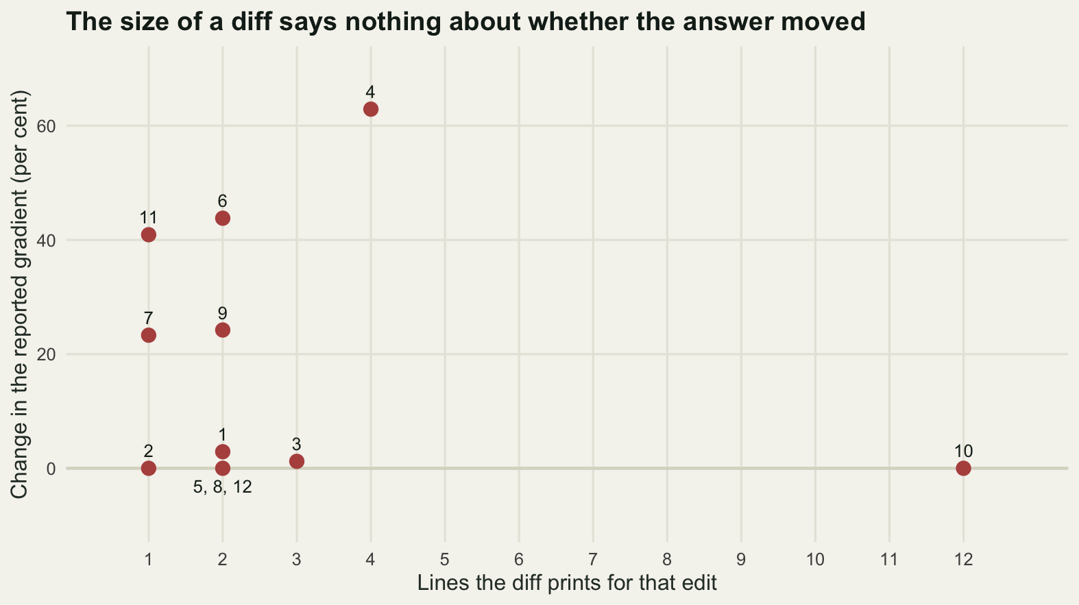
Twelve edits, 34 lines of diff in total, against a final file of 17 lines. The whole history is twice the size of the thing it is a history of, which is why keeping it costs nothing worth worrying about.
The scatter is the point of the section. The largest diff in the project prints 12 lines and changes the reported gradient by 0 per cent: it renames d to sur. Two of the three edits whose diff is a single line change it by 23.313 and 40.9109 per cent, because inserting one row filter is one line. The smallest diff that changed anything prints 1 line. There is no reading of the diff sizes that separates the five edits which moved nothing, three of them sharing a single point at two lines of diff, from the seven which did, and that is a general fact rather than a feature of this history: the size of a text change and the size of its effect on an estimate are measuring different things.
A line diff is a tool for text, and the reason that matters is the data file. A csv is text, so it diffs, but only if the lines stay where they are. The next block takes the first two hundred records of the counts file and compares three versions of it with the same comparator: the file after the late season visits were added, the same file with its rows in a different order, and the same file with a single count corrected.
as_lines <- function(z, n = 200)
  sprintf("%s,%s,%s,%d", z$patch[1:n], z$species[1:n], z$guild[1:n], z$count[1:n])

set.seed(11)
base_lines <- as_lines(d2)
late_lines <- as_lines(d3)
shuffled   <- base_lines[sample(length(base_lines))]
one_fix    <- base_lines
one_fix[57] <- sub(",[0-9]+$", ",9", one_fix[57])

round(c(records_compared = length(base_lines),
        records_the_late_visits_changed = sum(base_lines != late_lines),
        diff_lines_for_the_late_visits = length(line_diff(base_lines, late_lines)),
        diff_lines_for_a_pure_reordering = length(line_diff(base_lines, shuffled)),
        records_a_reordering_changed = sum(sort(base_lines) != sort(shuffled)),
        diff_lines_for_one_corrected_count = length(line_diff(base_lines, one_fix))), 4)
records_compared records_the_late_visits_changed
200 27
diff_lines_for_the_late_visits diff_lines_for_a_pure_reordering
54 352
records_a_reordering_changed diff_lines_for_one_corrected_count
0 2 Adding the late visits changed 27 of the 200 records and prints a diff of 54 lines, which is exactly what you want from a history: two lines per changed record, the old and the new, with the patch and the species on them. Correcting a single count prints 2 lines. Reordering the rows changes nothing at all, 0 records differ once both files are sorted, and the diff prints 352 lines, which is most of the file. Anybody reading that history sees a rewrite where nothing happened.
The practical consequence is that a data file under version control wants to be text, sorted in a fixed order, and written by something that does not reorder it on a whim. The same argument explains why a compressed archive or a spreadsheet workbook is a poor citizen of a repository: the bytes change everywhere for a change anywhere, so every commit is a full rewrite and the diff never says anything.
The last column of the earlier table is the one to act on. Each edit invalidates some of the figures already drawn, in the sense that redrawing one after the edit gives a different number, and over the twelve edits that comes to 28 figure redraws. The eleventh edit alone, one line dropping the flooded patch, invalidates all 7 figures drawn before it. In a project with a commit history you can answer that question after the fact, by checking out the state each figure came from and comparing. Without one you cannot, and the practical consequence is that the manuscript keeps whichever figures nobody happened to redraw.
The commands, and what does not belong in them
Six commands cover the whole of what this post has been measuring. They are not run here because this post has to render with nothing installed beyond ggplot2, and because a version control system is a thing you run in a terminal in a project folder rather than inside a document:
git init                                  # start recording this folder
git status                                # what has changed since the last commit
git add analysis.R patch_counts.csv       # choose what goes in the next commit
git commit -m "rarefy to 40 individuals"  # record a state, with a message
git log --oneline                         # list the states, newest first
git checkout 4f2a1c9 -- analysis.R        # bring one file back from one state
Two of those deserve a second look. git add is the step that surprises people who expect the tool to save everything: you choose what the commit contains, which means a commit can be a coherent change rather than whatever happened to be on disk at five o’clock. And git checkout with a commit name in front of it is the whole of the reconstruction measured in this post. It is the command that turns “which state of the code produced this figure” from a question about your memory into a question about a recorded fact.
The list of what to leave out belongs in a file called .gitignore, one pattern per line, and it is worth writing on the first day rather than after the repository has doubled in size:
_output/
*.rds
*.tif
raw_audio/
.Rhistory
The message matters more than the mechanics. git log on this project would print thirteen lines, one for the first version and one for each edit, and the difference between a history you can use and one you cannot is whether those lines say “rarefaction depth 30 to 40” or “update”. A commit message is the only place in the whole system where the reason for an edit is recorded, since the diff shows what changed and never why.
Recording the data file is the part of the practice ecologists get wrong in both directions. The counts file in this post is a small text file that changed three times, and putting it under version control is what turns the data version from an unrecorded fact into a recoverable one: that is the difference between the two of eight and the five of eight in the section above. What does not belong is the material that is large, binary, or regenerable. A raw acoustic archive, a folder of camera trap images, a several gigabyte raster: version control stores a complete copy of every version of every file, so a binary file that changes weekly grows the repository without ever producing a readable diff. Generated output has the opposite problem: figures, fitted model objects and intermediate .rds files can be rebuilt from the code and the data, and committing them means the history records the same result twice and invites the two copies to disagree.
The seed is the third component and it belongs in the script, not in a note. set.seed(20260817) on the line above the resampling makes the seed part of the code state, which means the commit that records the code records the seed for free. That is not what this history did: the seed of each seeded figure is known only because the provenance table records it, and two of the four come back only once that seed is supplied on top of the code and the data. Figure six has no recorded seed at all, so nothing brings it back.
The honest limit
This post measures one file and one person. Both are simplifications, and the second is the larger one. Most of what a version control system is built for is two people editing the same file at once, which produces a class of problem the measurement here never reaches: a merge, a conflict, and the question of which of two edits to the same line survives. A commit is also atomic across files, which is the property that makes it a record of a state of the project rather than of a script, and a one file history cannot show that either. What a solo ecologist gets from the tool is the part measured above, and it is enough on its own to be worth the afternoon.
The measurement in this post is a reconstruction test, and reconstruction is not correctness. All seven figures that come back come back to the last digit, and nothing in that says any of them answers the right question. Figure one reports a gradient of 8.5531 from the uncorrected data file, with four counts inflated tenfold, and it is perfectly reproducible: the reproduction is of an answer that a data check later rejected. A commit history is a record of what you did, and it is neither an argument that what you did was sensible nor a substitute for checking an analysis script.
The second limit is granularity, and it decides whether the code state is available for every figure at all rather than for some of them. A commit for every edit puts all 8 figure states in the history. Commit twice a week instead, after three or four edits have accumulated, and the states in between are as gone as they were under the naming scheme: the surviving figure states in this history drop to between 1 and 4 depending on where the commits happen to fall.
gran <- sapply(1:6, function(k) sum(figs$code %in% unique(c(seq(0, 12, by = k), 12))))
names(gran) <- paste0("every_", 1:6)
print(gran)
every_1 every_2 every_3 every_4 every_5 every_6
8 3 4 2 1 2 round(c(figure_states = nrow(figs),
with_a_commit_per_edit = gran[["every_1"]],
fewest_across_coarser_schedules = min(gran[-1]),
most_across_coarser_schedules = max(gran[-1])), 4) figure_states with_a_commit_per_edit
8 8
fewest_across_coarser_schedules most_across_coarser_schedules
1 4 Which of the coarser schedules does best is not a fact about commit frequency, it is an accident of whether the commit points happen to coincide with the days figures were drawn. That is the real argument for committing at every edit that changes an answer: you cannot know in advance which state somebody will need, so the only reliable policy is to keep them all.
The third limit is the one this post shares with the rest of the cluster. Version control records the code, and if you commit it, the data. It does not record the versions of the packages the script loaded, which is what pinning package versions with renv is for, and it does not record the R version, the operating system or the numerical libraries underneath. A perfect commit history plus a lockfile plus a recorded seed answers “which state of the code produced this figure” and leaves “will this state of the code still produce that figure in five years” open. The two questions are different, and only the first one has a cheap answer.
Where to go next
The cheapest thing to do after reading this is not to learn the commands. It is to put a set.seed above every random step in the script you are working on this week and to commit the data file next to the code, because those are the two of the three components that most projects are missing and the ones that stand between the 2 of 8 and the 7 of 8 measured here. After that, a reproducible statistical workflow in R is the project layout that makes a commit history worth having, and checking an analysis script is the set of checks that tell you whether a state you have recovered actually runs.
Once the history exists it changes what the neighbouring craft is for. Testing your analysis code becomes a way to find out which commit broke something rather than only that something is broken, and turning your code into an R package is the natural next step when the same function starts appearing in two repositories, because a package has a version number and a version number is a commit you can name.
References
Wilson G, Bryan J, Cranston K, Kitzes J, Nederbragt L, Teal TK 2017 PLoS Computational Biology 13(6):e1005510 (10.1371/journal.pcbi.1005510)
Ram K 2013 Source Code for Biology and Medicine 8(1):7 (10.1186/1751-0473-8-7)
Blischak JD, Davenport ER, Wilson G 2016 PLoS Computational Biology 12(1):e1004668 (10.1371/journal.pcbi.1004668)
Sandve GK, Nekrutenko A, Taylor J, Hovig E 2013 PLoS Computational Biology 9(10):e1003285 (10.1371/journal.pcbi.1003285)
Perez-Riverol Y, Gatto L, Wang R, Sachsenberg T, Uszkoreit J, Leprevost FV, Fufezan C, Ternent T, Eglen SJ, Katz DS, Pollard TJ, Konovalov A, Flight RM, Blin K, Vizcaino JA 2016 PLoS Computational Biology 12(7):e1004947 (10.1371/journal.pcbi.1004947)
Myers EW 1986 Algorithmica 1(1-4):251-266 (10.1007/BF01840446)