library(ggplot2)

te_pal <- list(forest = "#275139", green = "#2f8f63", sage = "#93a87f",
               clay = "#b5534e", gold = "#cda23f", line = "#dad9ca",
               ink = "#16241d", paper = "#f5f4ee")

theme_te <- function() {
  theme_minimal(base_size = 12) +
    theme(panel.grid.minor = element_blank(),
          panel.grid.major = element_line(colour = "#e7e6dc"),
          plot.background = element_rect(fill = "#f5f4ee", colour = NA),
          panel.background = element_rect(fill = "#f5f4ee", colour = NA),
          plot.title = element_text(face = "bold", colour = te_pal$ink),
          axis.title = element_text(colour = "#2c3a31"))
}Speeding up your analysis code
R
reproducibility
ecology tutorial
ggplot2
Measure before you optimise: which R rewrites buy a constant factor, which change the algorithm, and what the time you save buys an ecological analysis.
The script has been running since Friday afternoon. It is Monday. It reads ten years of pitfall trapping, attaches the treatment and the trapping effort to every sample, standardises the catches, builds a site by site dissimilarity matrix, and bootstraps the difference in beetle density between grazed and ungrazed grassland. The plan was to run it four times, once per definition of grazing, before the manuscript goes out on Thursday. Nobody has measured where the time goes. The guess in the room is the bootstrap, because 999 resamples sounds like the expensive part, and the second guess is the dissimilarity matrix, because it is the biggest object in the workspace.
Both guesses are wrong, and this post measures by how much. It also measures three rewrites everybody reaches for: replacing a loop with a vectorised call, replacing a search with a lookup, and pre-allocating a vector instead of growing it. They are not the same kind of thing at all. The first buys a constant factor and then stops improving, however much data you give it. The other two change the algorithm, and their advantage keeps growing with the size of the survey. Telling the two kinds apart before you spend an afternoon on the wrong one is most of the skill.
There is one rule that runs through everything below. Absolute seconds are not reportable. A second on the machine that rendered this page means nothing on yours: different processor, different memory, different R build, different load from whatever else the machine is doing. So every timing below is given as a ratio between two timings taken in the same session, minutes apart, which is the most portable form a statement about speed has. It is not a fully portable form, and the last section is about where it fails. Every ratio on this page is measured again each time the page is built, so the digits you are reading were taken on whatever machine built it, and they are worth one or two significant figures at most, whatever the printed output carries, because nothing past that is a property of the code. This is the same portability question as never asking the machine what time zone it is in: an analysis that reports something about its own hardware is reporting something the reader cannot use.
The claim at the end is ecological rather than computational. The time saved is not saved for its own sake. It buys resamples, and the number of resamples decides how much of the confidence interval you report is data and how much is the random number generator. Where checking an analysis script asks whether a script gives the same answer twice, this post asks what it costs to make the answer stable enough to be worth reporting.
A timer you can trust in twenty lines
system.time is the whole timing apparatus base R gives you, and used naively it is close to useless. Two problems. The first is resolution: an operation that takes a fifth of a millisecond registers as zero, and a ratio with a zero in the denominator is not a measurement. The second is noise: the same expression timed twice differs by a few per cent because of the operating system’s scheduler, and by much more if a garbage collection happens to land inside one of the two runs.
Both problems have the same fix, and it is the fix every serious benchmarking package uses. Run the expression enough times that the total is comfortably above the clock’s resolution, divide by the number of runs, repeat that whole block several times, and keep the fastest block. The fastest block is the right summary rather than the mean, because everything that goes wrong during a timing makes it slower and nothing makes it faster: the minimum is the closest thing to the cost of the work itself.
bench <- function(expr, blocks = 5, budget = 0.15) {
  e <- substitute(expr)
  p <- parent.frame()
  reps <- 1L
  el <- 0
  repeat {
    el <- system.time(for (r in seq_len(reps)) eval(e, p))[["elapsed"]]
    if (el > 0.02 || reps >= 1e6) break
    reps <- 4L * reps
  }
  reps <- max(1L, as.integer(ceiling(reps * budget / el)))
  t <- numeric(blocks)
  for (b in seq_len(blocks)) {
    t[b] <- system.time(for (r in seq_len(reps)) eval(e, p))[["elapsed"]] / reps
  }
  structure(min(t), reps = reps, spread = max(t) / min(t))
}

bench_lines <- length(deparse(bench))
c(bench_lines = bench_lines)
bench_lines
20 x <- as.numeric(1:20000)
add_up <- function(v) {
s <- 0
for (i in seq_along(v)) s <- s + sqrt(v[i])
s
}
fast <- bench(sum(sqrt(x)))
slow <- bench(add_up(x))
report_ratio <- function(a, b) signif(as.numeric(a) / as.numeric(b), 1)
c(the_two_agree = isTRUE(all.equal(sum(sqrt(x)), add_up(x))))the_two_agree
TRUE print(c(repetitions_for_the_vectorised_call = attr(fast, "reps"),
repetitions_for_the_loop = attr(slow, "reps")))repetitions_for_the_vectorised_call repetitions_for_the_loop
2439 260 print(round(c(block_spread_vectorised = attr(fast, "spread"),
block_spread_loop = attr(slow, "spread")), 3))block_spread_vectorised block_spread_loop
1.027 1.007 c(loop_over_vectorised = report_ratio(slow, fast))loop_over_vectorised
10 The calibration loop is doing the work that makes the rest of the post possible. Timing sum(sqrt(x)) once would return zero, because it finishes well inside the resolution of the clock; the timer quadruples the repetition count until a block lasts long enough to measure, then scales it to the time budget. On the machine that built this page it settled on 2439 runs of the vectorised call per block and 260 runs of the loop over the same 20000 numbers, and those two counts are the first thing on the page that would come out differently somewhere else. The two return the same answer, which the chunk checks. They are one computation written two ways, and the ratio between them is the shape of everything that follows.
The block spread printed above is the slowest block divided by the fastest, and it is the honest measure of how much a single timing can be trusted. On the build you are reading, the worse of the two was 1.03. A spread near one says the machine was quiet while the blocks ran and the fastest block is a clean reading; a spread well above one says something else was competing for the processor, and every ratio taken on that build is worth fewer digits than it appears to have. It is the first number to read on a timing page, including this one, and it is why every ratio below is worth one or two significant figures at most, however many digits happen to be printed.
Two things this timer deliberately does not do. It does not stop the garbage collector, and it does not measure memory. Both are visible in the block spread when they matter, and both are mentioned again in the last section, because the vectorised versions below win on time by spending memory.
For real work you would not write this. Base R ships Rprof, which interrupts the interpreter a few hundred times a second and records the call stack, so it tells you which function the time is in rather than which stage. The profvis package draws the result as a flame graph, and bench::mark does what bench above does with better statistics and a check that the two expressions return the same value. None of them is run here, because this post has to render with nothing installed beyond ggplot2, and because Rprof writes its output to a file:
# not run here: Rprof writes a file, and profvis is a package this blog does not install
Rprof("profile.out", interval = 0.005, line.profiling = TRUE)
site_summary(records, sites)
Rprof(NULL)
summaryRprof("profile.out", lines = "show")$by.self[1:8, ]

profvis::profvis(site_summary(records, sites))
bench::mark(loop_version(m), vector_version(m), iterations = 20)
The survey the script is analysing
Everything below is measured on one simulated monitoring scheme, so that the ecological answer is known and the computational question has somewhere real to land. Sites are visited repeatedly, every visit produces one record with a trap effort and a beetle catch, and a small fraction of the visits have zero trap nights because the trap was lost or flooded. Site level attributes, the grazing treatment and a relative effort correction, live in a separate table keyed by site code, which is how field data almost always arrives.
set.seed(20260812)

n_site <- 480
n_spec <- 25
n_rec <- 24000

site_code <- sprintf("P%04d", seq_len(n_site))
treat <- rep(c("grazed", "ungrazed"), length.out = n_site)
effort <- round(runif(n_site, 0.7, 1.4), 2)

rec_site <- sample(site_code, n_rec, replace = TRUE)
rec_nights <- sample(c(0, 4, 5, 6, 7, 8, 10, 12), n_rec, replace = TRUE,
                     prob = c(0.02, rep(0.14, 7)))
site_rate <- ifelse(treat == "grazed", 3.6, 2.4) * exp(rnorm(n_site, 0, 0.45))
rec_catch <- rpois(n_rec,
                   site_rate[match(rec_site, site_code)] *
                     effort[match(rec_site, site_code)] * pmax(rec_nights, 1))
comm <- matrix(rpois(n_site * n_spec, 3), n_site, n_spec)

round(c(sites = n_site,
        species = n_spec,
        sample_records = n_rec,
        visits_per_site = n_rec / n_site,
        records_with_no_trap_nights = sum(rec_nights == 0),
        median_catch = median(rec_catch),
        largest_catch = max(rec_catch)), 4)
sites species
480 25
sample_records visits_per_site
24000 50
records_with_no_trap_nights median_catch
524 20
largest_catch
197 Fifty visits per site is a large scheme but not an unusual one; ten seasons with five trapping rounds in each gets there. The community matrix is separate, one row per site and one column per morphospecies, and it is the input to the dissimilarity stage.
Two rewrites, and only one of them keeps paying
The first computation is the pairwise Bray-Curtis dissimilarity between sites, which is the standard input to an ordination or a PERMANOVA. Three versions, all returning the same matrix. The first loops over site pairs and then over species, which is how the formula reads. The second loops over site pairs but does the species sum with a vectorised call. The third loops over species and does every site pair at once with outer, which is a different shape of computation entirely: 25 iterations instead of nearly twenty thousand.
bray_triple <- function(m) {
  n <- nrow(m)
  ns <- ncol(m)
  d <- matrix(0, n, n)
  for (i in seq_len(n - 1)) {
    for (j in (i + 1):n) {
      num <- 0
      den <- 0
      for (k in seq_len(ns)) {
        num <- num + abs(m[i, k] - m[j, k])
        den <- den + m[i, k] + m[j, k]
      }
      d[i, j] <- num / den
      d[j, i] <- d[i, j]
    }
  }
  d
}

bray_pairs <- function(m) {
  n <- nrow(m)
  d <- matrix(0, n, n)
  for (i in seq_len(n - 1)) {
    for (j in (i + 1):n) {
      d[i, j] <- sum(abs(m[i, ] - m[j, ])) / sum(m[i, ] + m[j, ])
      d[j, i] <- d[i, j]
    }
  }
  d
}

bray_vec <- function(m) {
  n <- nrow(m)
  num <- matrix(0, n, n)
  for (k in seq_len(ncol(m))) {
    num <- num + abs(outer(m[, k], m[, k], "-"))
  }
  num / outer(rowSums(m), rowSums(m), "+")
}

check <- comm[1:40, ]
c(pairs_agrees_with_triple = isTRUE(all.equal(bray_triple(check), bray_pairs(check))),
  vec_agrees_with_triple = isTRUE(all.equal(bray_triple(check), bray_vec(check))))
pairs_agrees_with_triple vec_agrees_with_triple
TRUE TRUE The agreement check is not decoration. A rewrite that is faster and wrong is the most expensive outcome available here, and the check costs one line. Speeding up an analysis is exactly the situation in which testing your analysis code earns its place: the old version is the golden test for the new one.
Now count the work before timing it. The triple loop runs one interpreted iteration per site pair per species. The pair loop runs one per site pair. The vectorised version runs one per species, whatever the number of sites. Those counts are exact arithmetic, not measurements, and they are the prediction the clock is about to be compared against.
bray_sizes <- c(50, 100, 200)
comms <- lapply(bray_sizes, function(n) comm[seq_len(n), ])

iter_counts <- data.frame(
  sites = bray_sizes,
  triple_loop = bray_sizes * (bray_sizes - 1) / 2 * n_spec,
  pair_loop = bray_sizes * (bray_sizes - 1) / 2,
  vectorised = rep(n_spec, length(bray_sizes)))
iter_counts$triple_over_vectorised <- iter_counts$triple_loop / iter_counts$vectorised
print(iter_counts)
sites triple_loop pair_loop vectorised triple_over_vectorised
1 50 30625 1225 25 1225
2 100 123750 4950 25 4950
3 200 497500 19900 25 19900bray_t <- t(sapply(comms, function(m)
c(triple = bench(bray_triple(m), blocks = 7),
pairs = bench(bray_pairs(m), blocks = 7),
vec = bench(bray_vec(m), blocks = 7))))
bray_ratio <- data.frame(
sites = bray_sizes,
triple_over_vec = round(bray_t[, "triple"] / bray_t[, "vec"], 1),
pairs_over_vec = round(bray_t[, "pairs"] / bray_t[, "vec"], 1),
triple_over_pairs = round(bray_t[, "triple"] / bray_t[, "pairs"], 1))
print(bray_ratio) sites triple_over_vec pairs_over_vec triple_over_pairs
1 50 6.5 3.1 2.1
2 100 7.2 3.4 2.1
3 200 8.2 4.0 2.1bray_mean_ratio <- report_ratio(mean(bray_ratio$triple_over_vec), 1)
bray_inner_only <- report_ratio(mean(bray_ratio$triple_over_pairs), 1)
bray_first <- bray_ratio$triple_over_vec[1]
bray_last <- bray_ratio$triple_over_vec[length(bray_sizes)]
c(iterations_saved_at_100_sites = iter_counts$triple_over_vectorised[2],
measured_ratio_over_the_three_sizes = bray_mean_ratio,
measured_inner_loop_only = bray_inner_only) iterations_saved_at_100_sites measured_ratio_over_the_three_sizes
4950 7
measured_inner_loop_only
2 At 100 sites the iteration count says the vectorised version should have 4950 times less to do than the triple loop. Averaged over the three sizes the clock says 7. That gap of nearly three orders of magnitude is the single most useful thing to understand about vectorising R code, and it is not a failure of the measurement.
Vectorising does not remove the arithmetic. Every one of the 497500 subtractions the 200 site problem needs still happens; they happen inside a compiled loop rather than inside the interpreter, so what disappears is the interpreter’s overhead per operation and nothing else. That overhead is a fixed number of nanoseconds spent working out what + means for these two objects, checking their types and lengths, and deciding where the answer goes. Doing it once per vector instead of once per element removes almost all of it, and there it stops: the arithmetic that remains is the same arithmetic. So the payoff is a constant factor, and once the factor is bought there is nothing left to buy. The table above shows exactly that. Across a fourfold increase in the number of sites the ratio moves only from 6.5 to 8.2, and the small rise it does show is the vectorised version’s own fixed costs becoming negligible rather than the loop getting relatively worse.
Vectorising the species loop alone, which is the change from bray_triple to bray_pairs, recovers a factor of 2 of that. The rest comes from also doing the site pairs at once, and that step is the one that changes what the code looks like: bray_vec does not contain the phrase “for each pair of sites” anywhere. It is a different way of writing the same formula, which is why the check that the three agree is not optional.
The second rewrite looks similar and is not. The script has to attach the treatment and the effort correction to each of the 24000 records, given a site table of 480 rows. The version people write searches the site table once per record with which. The version R intends is match, which builds a hash table over the site codes once and then looks each record up in constant time.
attach_scan <- function(codes, table_codes, table_value) {
  out <- numeric(length(codes))
  for (i in seq_along(codes)) {
    out[i] <- table_value[which(table_codes == codes[i])[1]]
  }
  out
}

attach_hash <- function(codes, table_codes, table_value) {
  table_value[match(codes, table_codes)]
}

lookup_sizes <- c(2000, 8000, 32000)
lookup <- t(sapply(lookup_sizes, function(n) {
  m <- n / 20
  tc <- sprintf("P%05d", seq_len(m))
  tv <- runif(m)
  codes <- sample(tc, n, replace = TRUE)
  ok <- isTRUE(all.equal(attach_scan(codes, tc, tv), attach_hash(codes, tc, tv)))
  c(records = n, sites = m, agree = ok,
    time_ratio = round(bench(attach_scan(codes, tc, tv), blocks = 7) /
                         bench(attach_hash(codes, tc, tv), blocks = 7), 1),
    comparison_ratio = round(n * m / (n + m), 1))
}))
print(as.data.frame(lookup))
records sites agree time_ratio comparison_ratio
1 2000 100 1 142.0 95.2
2 8000 400 1 258.0 381.0
3 32000 1600 1 656.9 1523.8n_look <- length(lookup_sizes)
c(scan_over_hash_at_the_smallest_size = unname(round(lookup[1, "time_ratio"])))scan_over_hash_at_the_smallest_size
142 c(comparison_ratio_multiplies_by =
round(unname(lookup[n_look, "comparison_ratio"] /
lookup[n_look - 1, "comparison_ratio"]), 4))comparison_ratio_multiplies_by
3.9995 panel_lab <- c("Bray-Curtis matrix: the same algorithm, less overhead",
"Attaching site attributes: a different algorithm")
rew <- rbind(
data.frame(size = bray_sizes, ratio = bray_ratio$triple_over_vec,
version = "Loop over pairs and species",
panel = panel_lab[1]),
data.frame(size = bray_sizes, ratio = bray_ratio$pairs_over_vec,
version = "Loop over pairs only",
panel = panel_lab[1]),
data.frame(size = lookup[, "records"], ratio = lookup[, "time_ratio"],
version = "Loop with which() per record",
panel = panel_lab[2]))
rew$panel <- factor(rew$panel, levels = panel_lab)
rew$version <- factor(rew$version,
levels = c("Loop over pairs and species",
"Loop over pairs only",
"Loop with which() per record"))
ggplot(rew, aes(size, ratio, colour = version, shape = version)) +
geom_hline(yintercept = 1, linetype = 2, colour = te_pal$sage, linewidth = 0.8) +
geom_line(linewidth = 0.9) +
geom_point(size = 3.2) +
facet_wrap(~panel, scales = "free_x") +
scale_x_log10() +
scale_y_log10(breaks = c(1, 3, 10, 30, 100, 300, 1000)) +
scale_colour_manual(values = c(te_pal$clay, te_pal$gold, te_pal$forest), name = NULL) +
scale_shape_manual(values = c(16, 17, 15), name = NULL) +
labs(x = "Sites (left panel) or sample records (right panel), log scale",
y = "Times slower than the\nvectorised version (log scale)",
title = "One rewrite stops paying, the other keeps paying") +
theme_te() +
theme(legend.position = "top",
strip.text = element_text(colour = te_pal$ink, face = "bold", size = 9))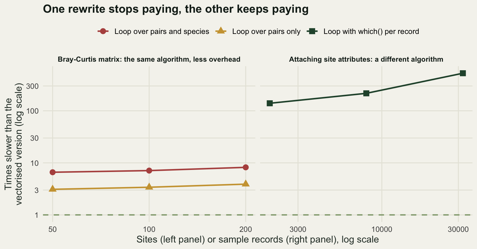
The lookup ratio starts near 142 at 2000 records and reaches 657 by 32000, and unlike the Bray-Curtis ratio it has not finished growing. The reason is in the comparison counts rather than in the clock. The scanning version compares every record against every site, so its work is the product of the two; match builds one hash table and then does work proportional to their sum. Quadrupling the size of the survey therefore multiplies the comparison ratio by 3.9995 and will go on doing so. At the largest size tested the scanning version makes 1523.8 comparisons for every one the hash version makes.
The measured time ratio and the comparison ratio need not agree, and the reason is worth knowing: hashing a string costs more than comparing one, so match pays a larger constant per unit of work. Constants are what the clock measures and counts are what the algorithm determines, and when the two disagree it is the count that says what happens next year. Only the clock is plotted in the figure; the counts sit in the table above it. The distance between the two is the constant, and nothing forces it to keep the same sign from one row of that table to the next. The count is the part that keeps climbing, and that is the algorithm.
This is the distinction the whole section exists for. Rewriting a loop as a vectorised call is a change of constant factor: worth doing, cheap to do, and finished once done. Replacing a scan with a lookup is a change of algorithm, and the bigger the data get the more it is worth. If you have one afternoon, spend it looking for the second kind. The first kind will still be there next week and will still be worth the same amount.
The vector that grows
The other rewrite everybody has heard of is pre-allocation. Growing a result with x <- c(x, new) inside a loop is the natural way to write it when you do not know how many results there will be, and it is the classic quadratic mistake: each c() allocates a fresh vector and copies everything accumulated so far into it.
The number of elements copied is exact arithmetic, so it can be stated before anything is timed. A loop that grows a vector to length n copies 1 element, then 2, and so on, which totals n times n plus one over two. Pre-allocating copies nothing: it writes each element once into space that already exists.
grow_it <- function(n) {
  x <- numeric(0)
  for (i in seq_len(n)) x <- c(x, i)
  x
}

prealloc_it <- function(n) {
  x <- numeric(n)
  for (i in seq_len(n)) x[i] <- i
  x
}

grow_sizes <- c(2500, 5000, 10000, 20000, 40000)
copies_grow <- grow_sizes * (grow_sizes + 1) / 2
copies_prealloc <- grow_sizes

c(agree = isTRUE(all.equal(grow_it(500), prealloc_it(500))))
agree
TRUE print(data.frame(length = grow_sizes,
elements_copied_growing = copies_grow,
elements_written_prealloc = copies_prealloc,
ratio = round(copies_grow / copies_prealloc, 1))) length elements_copied_growing elements_written_prealloc ratio
1 2500 3126250 2500 1250.5
2 5000 12502500 5000 2500.5
3 10000 50005000 10000 5000.5
4 20000 200010000 20000 10000.5
5 40000 800020000 40000 20000.5log_slope <- function(y, x) coef(lm(log(y) ~ log(x)))[[2]]
round(c(exact_slope_growing = log_slope(copies_grow, grow_sizes),
exact_slope_prealloc = log_slope(copies_prealloc, grow_sizes)), 4) exact_slope_growing exact_slope_prealloc
1.9999 1.0000 grow_t <- sapply(grow_sizes, function(n) bench(grow_it(n), blocks = 4))
prealloc_t <- sapply(grow_sizes, function(n) bench(prealloc_it(n), blocks = 4))
grow_slope <- log_slope(grow_t, grow_sizes)
prealloc_slope <- log_slope(prealloc_t, grow_sizes)
n_grow <- length(grow_sizes)
grow_ref <- min(c(grow_t, prealloc_t))
grow_rel <- grow_t / grow_ref
prealloc_rel <- prealloc_t / grow_ref
grow_gap <- report_ratio(grow_t[n_grow], prealloc_t[n_grow])
round(c(measured_slope_growing = grow_slope,
measured_slope_prealloc = prealloc_slope), 1) measured_slope_growing measured_slope_prealloc
2 1 c(ratio_at_the_largest_size = grow_gap)ratio_at_the_largest_size
2000 grow_df <- rbind(
data.frame(length = grow_sizes, rel = grow_rel,
version = "Grown with c() in the loop"),
data.frame(length = grow_sizes, rel = prealloc_rel,
version = "Pre-allocated, then filled"))
grow_df$version <- factor(grow_df$version,
levels = c("Grown with c() in the loop",
"Pre-allocated, then filled"))
ggplot(grow_df, aes(length, rel, colour = version, shape = version)) +
geom_line(linewidth = 0.9) +
geom_point(size = 3.2) +
scale_x_log10(breaks = grow_sizes) +
scale_y_log10(breaks = c(1, 3, 10, 30, 100, 300, 1000, 3000, 10000)) +
scale_colour_manual(values = c(te_pal$clay, te_pal$forest), name = NULL) +
scale_shape_manual(values = c(16, 15), name = NULL) +
labs(x = "Final length of the vector (log scale)",
y = "Time relative to the fastest\nmeasurement here (log scale)",
title = sprintf("Growing a vector costs a slope of %.1f, pre-allocating %.1f",
grow_slope, prealloc_slope)) +
theme_te() +
theme(legend.position = "top")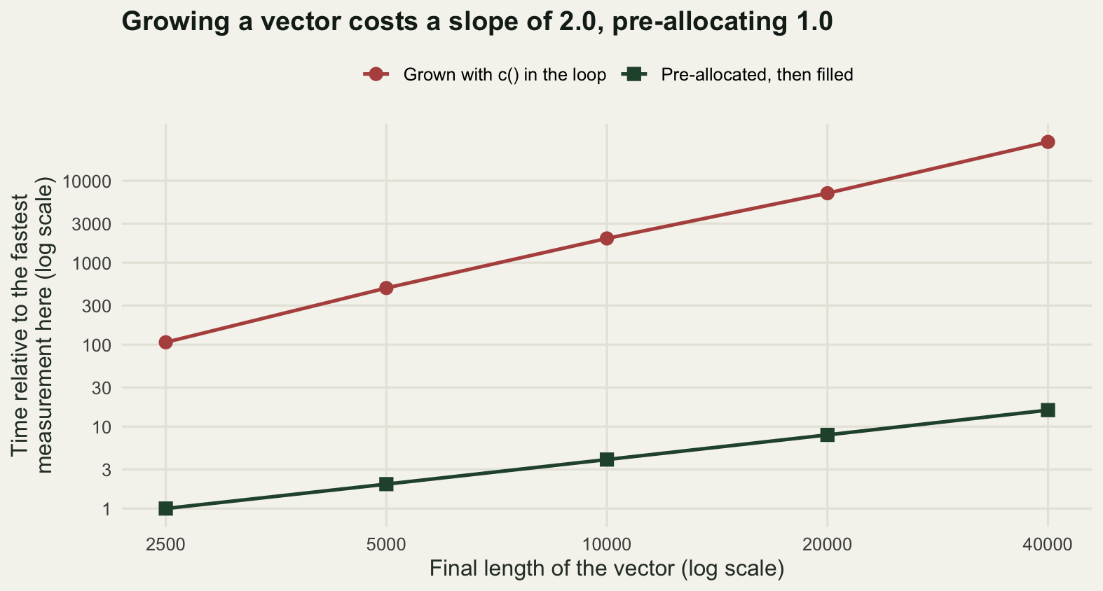
At the largest size tested the grown version is about 2000 times slower, but the ratio is not the finding. The two log-log slopes are. The pre-allocated version has a measured slope of 1.0: double the length, double the cost, which is what a loop doing one thing per element must do. The grown version has a measured slope of 2.0, and a slope above one means the cost per element is itself rising with the length of the vector.
The exact copy count gives a slope of 1.9999, and the measured one lands near it rather than on it. The gap is worth a sentence rather than an apology. Copying a long vector is not the same cost per element as copying a short one: a long copy runs at the memory system’s streaming speed while a short one is dominated by the cost of the allocation that precedes it. So the clock reads a slightly different exponent from the one the arithmetic predicts, and it will read a different one again on your machine, because that number is a property of a memory hierarchy rather than of the code.
The direction is not in doubt, and the direction is what matters. 800020000 elements are copied to build a vector of 40000 numbers, against 40000 written when the space is allocated first. That ratio of 20000.5 is not a constant factor and it does not stop growing: it is half the length of the vector. This is why a loop that felt tolerable on a pilot data set becomes impossible on the full one, and why the fix is worth applying before you find out.
The practical form of the fix is not always numeric(n). When the number of results is genuinely unknown, allocate generously and trim at the end, or collect the pieces in a list and call unlist or do.call(rbind, ...) once, which copies everything exactly once rather than once per iteration. What you must not do is let the loop body extend the result.
Where the time actually is
Now the script itself, in six stages, each one timed separately. Attaching the site attributes to the records, converting catches to a density per hundred trap nights, averaging up to the site, building the dissimilarity matrix, bootstrapping the grazing effect with 999 resamples, and fitting the summary model. The stages are ordinary code; the only thing that has been done to them is that each is a function so it can be timed on its own.
attach_naive <- function() {
  tr <- character(n_rec)
  ef <- numeric(n_rec)
  for (i in seq_len(n_rec)) {
    k <- which(site_code == rec_site[i])[1]
    tr[i] <- treat[k]
    ef[i] <- effort[k]
  }
  list(tr = tr, ef = ef)
}

attach_fast <- function() {
  k <- match(rec_site, site_code)
  list(tr = treat[k], ef = effort[k])
}

densities <- function(att) {
  keep <- rec_nights > 0
  list(dens = 100 * rec_catch[keep] / (rec_nights[keep] * att$ef[keep]),
       site = rec_site[keep])
}

site_means <- function(rates) {
  m <- tapply(rates$dens, rates$site, mean)
  as.numeric(m[site_code])
}

boot_effect <- function(x, g, b) {
  ig <- which(g == "grazed")
  iu <- which(g == "ungrazed")
  rowMeans(matrix(x[sample(ig, length(ig) * b, replace = TRUE)], b)) -
    rowMeans(matrix(x[sample(iu, length(iu) * b, replace = TRUE)], b))
}

att0 <- attach_fast()
rates0 <- densities(att0)
site_dens <- site_means(rates0)

round(c(records_kept = length(rates0$dens),
        sites_with_no_usable_record = sum(is.na(site_dens)),
        mean_density_grazed = mean(site_dens[treat == "grazed"]),
        mean_density_ungrazed = mean(site_dens[treat == "ungrazed"]),
        observed_effect = mean(site_dens[treat == "grazed"]) -
          mean(site_dens[treat == "ungrazed"])), 4)
records_kept sites_with_no_usable_record
23476.0000 0.0000
mean_density_grazed mean_density_ungrazed
385.8016 264.9530
observed_effect
120.8486 stage_name <- c("Attach site attributes", "Catch to density", "Average to sites",
"Dissimilarity matrix", "Bootstrap, 999 resamples", "Summary model")
stage_t <- c(bench(attach_naive(), blocks = 4),
bench(densities(att0), blocks = 4),
bench(site_means(rates0), blocks = 4),
bench(bray_vec(comm), blocks = 4),
bench(boot_effect(site_dens, treat, 999), blocks = 4),
bench(coef(lm(site_dens ~ treat)), blocks = 4))
stage_share <- 100 * stage_t / sum(stage_t)
stage_ceiling <- 1 / (1 - stage_t / sum(stage_t))
stage_gain <- 100 * (stage_ceiling - 1)
stages <- data.frame(stage = stage_name,
share_percent = round(stage_share, 1),
best_speed_up = round(stage_ceiling, 2),
gain_percent = round(stage_gain, 1))
print(stages[order(-stage_share), ]) stage share_percent best_speed_up gain_percent
1 Attach site attributes 56.5 2.30 129.8
4 Dissimilarity matrix 35.0 1.54 53.9
5 Bootstrap, 999 resamples 6.3 1.07 6.8
3 Average to sites 1.6 1.02 1.6
2 Catch to density 0.3 1.00 0.3
6 Summary model 0.2 1.00 0.2small_three <- sum(stage_share[c(2, 3, 6)])
round(c(attach_share = stage_share[1],
dissimilarity_share = stage_share[4],
bootstrap_share = stage_share[5],
the_other_three_together = small_three), 1) attach_share dissimilarity_share bootstrap_share
56.5 35.0 6.3
the_other_three_together
2.2 The stage that holds the run is the one nobody would name: attaching the site attributes takes 56 per cent of it on this build. The dissimilarity matrix, the biggest object in the workspace, takes 35 per cent. The bootstrap, the stage the room agreed was the expensive part, takes 6 per cent, and the three remaining stages together account for 2 per cent between them.
The two speed-up columns are the arithmetic that turns those shares into a decision, and they are Amdahl’s argument in one line. If a stage is a fraction p of the running time, then making that stage take no time at all speeds the whole script up by 1 over 1 minus p, and no rewrite of that stage, however clever, can do better; the last column says the same thing as the percentage gain that is on the table, which is what the following figure plots. Making the bootstrap instantaneous, by any means at all, could not make this script faster than 1.1 times. Somebody could spend two days rewriting it in C and produce a change nobody would notice. Fixing the attachment line, which is one call to match in place of one loop, has a ceiling of 2.3.
That is the argument for measuring before rewriting, and it does not depend on the particular numbers. It depends only on the fact that a script’s time is not spread evenly over its lines, and that people are bad at guessing where it collects. The stage that looks expensive is the one with a large number written in it.
whole_slow <- function() {
  att <- attach_naive()
  rates <- densities(att)
  g <- site_means(rates)
  bray_vec(comm)
  boot_effect(g, treat, 999)
  coef(lm(g ~ treat))
}

whole_fast <- function() {
  att <- attach_fast()
  rates <- densities(att)
  g <- site_means(rates)
  bray_vec(comm)
  boot_effect(g, treat, 999)
  coef(lm(g ~ treat))
}

c(same_answer = isTRUE(all.equal(attach_naive()$tr, attach_fast()$tr)))
same_answer
TRUE t_slow <- bench(whole_slow(), blocks = 4)
t_fast <- bench(whole_fast(), blocks = 4)
whole_gain <- as.numeric(t_slow / t_fast)
round(c(measured_whole_script_speed_up = whole_gain,
predicted_from_the_stage_table = 1 / (1 - stage_t[1] / sum(stage_t))), 1)measured_whole_script_speed_up predicted_from_the_stage_table
2.3 2.3 c(ceiling_if_the_bootstrap_stage_were_free = round(stage_ceiling[5], 1))ceiling_if_the_bootstrap_stage_were_free
1.1 stage_lab <- c("Share of the running time (per cent)",
"Whole script gain available (per cent)")
prof_df <- rbind(
data.frame(stage = stage_name, value = stage_share, panel = stage_lab[1]),
data.frame(stage = stage_name, value = stage_gain, panel = stage_lab[2]))
prof_df$panel <- factor(prof_df$panel, levels = stage_lab)
prof_df$stage <- factor(prof_df$stage, levels = stage_name[order(stage_share)])
prof_df$role <- factor(ifelse(prof_df$stage == "Attach site attributes",
"The line nobody suspects", "Every other stage"),
levels = c("The line nobody suspects", "Every other stage"))
ggplot(prof_df, aes(value, stage, fill = role)) +
geom_col(width = 0.66) +
geom_text(aes(label = sprintf("%.1f", value)),
hjust = -0.12, size = 3.1, colour = te_pal$ink) +
facet_wrap(~panel, scales = "free_x") +
scale_fill_manual(values = c(te_pal$clay, te_pal$forest), name = NULL) +
scale_x_continuous(expand = expansion(mult = c(0, 0.28))) +
labs(x = NULL, y = NULL,
title = "The expensive stage is not one of the two you would name") +
theme_te() +
theme(legend.position = "top",
plot.margin = margin(5.5, 15, 5.5, 5.5),
strip.text = element_text(colour = te_pal$ink, face = "bold", size = 9))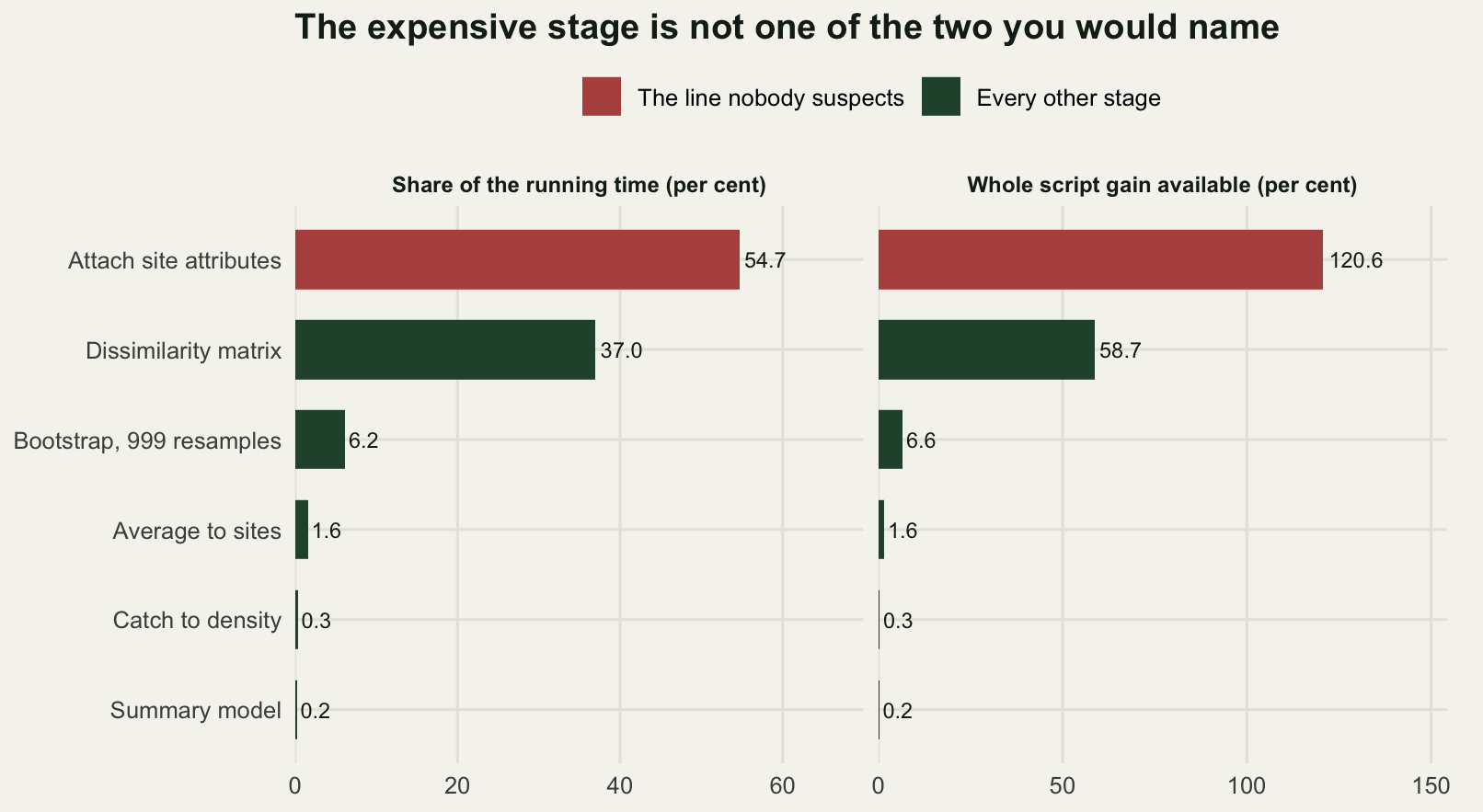
Running the whole script both ways confirms the arithmetic: replacing the loop with match makes it 2.3 times faster end to end, close to what the stage table predicted from the share that one stage held. The two do not have to agree exactly, and where they differ the gap is instructive rather than embarrassing. A stage timed on its own does not cost what it costs inside a pipeline that has already filled memory with the objects the earlier stages produced, and the timer ran each stage many times in a row, which is the friendliest possible case a processor cache will ever see. Stage timing is a map, not a survey. It is accurate enough to tell you where to go and not accurate enough to tell you what you will find when you get there.
The general lesson is not that lookups are slow. It is that the intuition about which stage is expensive was wrong by an order of magnitude, in a script of six stages that fits on one screen, written by somebody who knew what they were doing. The stage that felt expensive was the one with the big number in it, 999 resamples, and 999 resamples of 480 numbers is nothing at all. The stage that was expensive was the one that read like bookkeeping.
What the saved time buys the ecology
None of this matters unless the time turns into something. It does, and this is where a computational post gets an ecological number. The bootstrap resample count is not a matter of taste: it sets how much of the confidence interval you report comes from the data and how much comes from the random number generator. A percentile interval from 199 resamples is an estimate of an interval, and it has its own sampling error.
Here the same bootstrap is run 40 times over on the same data, changing nothing but the state of the random number generator, at three resample counts. If the reported interval were a property of the data, the 40 runs would agree.
boot_ci <- function(x, g, b) {
  ig <- which(g == "grazed")
  iu <- which(g == "ungrazed")
  d <- rowMeans(matrix(x[sample(ig, length(ig) * b, replace = TRUE)], b)) -
    rowMeans(matrix(x[sample(iu, length(iu) * b, replace = TRUE)], b))
  unname(quantile(d, c(0.025, 0.975)))
}

set.seed(9012)
b_grid <- c(199, 999, 4999)
n_repeat <- 40
ci_runs <- lapply(b_grid, function(b)
  t(sapply(seq_len(n_repeat), function(r) boot_ci(site_dens, treat, b))))

boot_tab <- do.call(rbind, lapply(seq_along(b_grid), function(i) {
  lo <- ci_runs[[i]][, 1]
  hi <- ci_runs[[i]][, 2]
  w <- mean(hi - lo)
  data.frame(resamples = b_grid[i],
             mean_width = round(w, 3),
             lower_bound_range = round(diff(range(lo)), 4),
             range_as_percent_of_width = round(100 * diff(range(lo)) / w, 4),
             sd_as_percent_of_width = round(100 * sd(lo) / w, 4))
}))
print(boot_tab)
resamples mean_width lower_bound_range range_as_percent_of_width
1 199 54.489 8.2560 15.1516
2 999 54.983 4.5263 8.2322
3 4999 55.848 2.0800 3.7245
sd_as_percent_of_width
1 3.8965
2 1.7211
3 0.8871round(c(spread_falls_by = boot_tab$sd_as_percent_of_width[1] /
boot_tab$sd_as_percent_of_width[3],
square_root_of_the_resample_ratio = sqrt(b_grid[3] / b_grid[1])), 4) spread_falls_by square_root_of_the_resample_ratio
4.3924 5.0120 offset <- seq(-0.28, 0.28, length.out = n_repeat)
boot_df <- do.call(rbind, lapply(seq_along(b_grid), function(i)
rbind(data.frame(x = i + offset, bound = ci_runs[[i]][, 1],
which_bound = "Lower 2.5 per cent bound"),
data.frame(x = i + offset, bound = ci_runs[[i]][, 2],
which_bound = "Upper 97.5 per cent bound"))))
boot_df$which_bound <- factor(boot_df$which_bound,
levels = c("Upper 97.5 per cent bound",
"Lower 2.5 per cent bound"))
ggplot(boot_df, aes(x, bound, colour = which_bound)) +
geom_point(size = 1.9, alpha = 0.9) +
scale_x_continuous(breaks = seq_along(b_grid), labels = b_grid) +
scale_colour_manual(values = c(te_pal$gold, te_pal$forest), name = NULL) +
labs(x = "Bootstrap resamples",
y = "Reported bound on the grazing effect\n(beetles per 100 trap nights)",
title = "The same script, run again, reports a different interval") +
theme_te() +
theme(legend.position = "top")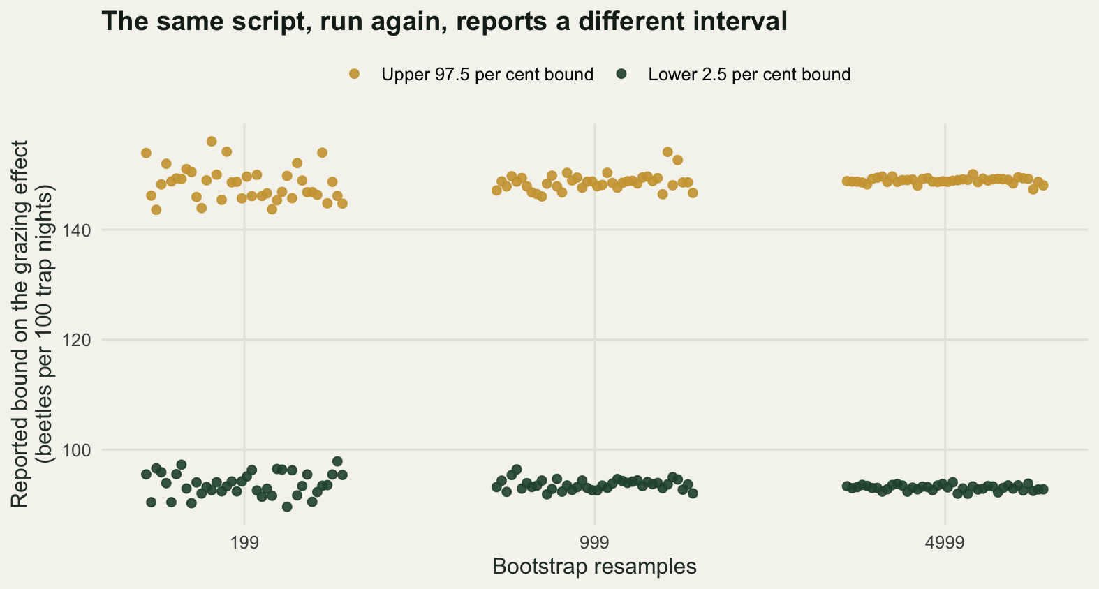
At 199 resamples the lower bound of the 95 per cent interval lands anywhere within a band 15.1516 per cent as wide as the interval itself, purely from the state of the random number generator. Two people running the identical script on the identical data write down different numbers. That is a tolerable amount of slop if the bound is nowhere near zero and a serious problem if it is, which is the only case anybody argues about.
At 999 resamples the band is 8.2322 per cent of the width and at 4999 it is 3.7245 per cent. The standard deviation of the reported bound falls from 3.8965 per cent of the width to 0.8871 per cent as the resample count goes up 25-fold, a factor of 4.3924 against the 5.0120 the square root law predicts, which is as close as 40 repeats can be expected to get. The interval width itself barely moves: 54.489 at the lowest resample count against 55.848 at the highest. It is not the width that is unstable, it is which particular value you happen to report.
Now join that to the profile.
boot_multiple <- as.numeric(stage_t[1] / stage_t[5])
boot_afforded <- 999 * (1 + boot_multiple)
round(c(bootstrap_multiples_the_wasted_time_would_pay_for = boot_multiple,
        resamples_for_the_same_wall_clock = boot_afforded), 1)
bootstrap_multiples_the_wasted_time_would_pay_for
8.9
resamples_for_the_same_wall_clock
9906.2 The time the naive attachment line was wasting, on its own, was worth 8.9 runs of the 999 resample bootstrap on this build. Spend it on resamples instead and the same wall clock affords about 9900 of them in place of 999, and the stability table says what that buys: the band the reported bound wanders in shrinks by roughly the square root of the increase. Nothing about the ecology changed, nothing about the data changed, and the number that goes in the abstract stopped depending on the seed.
That is the argument for caring about any of this. The script does not become correct by becoming fast. It becomes affordable to run at a setting where the answer stops depending on the seed, and the setting the slow version could afford was the setting that made the interval unstable. Power analysis by simulation in R runs into the same wall from the other side: a power curve needs thousands of simulated data sets, and a slow inner loop is the reason people report a power curve built from 100.
The honest limit
Rewriting pays only when the analysis repeats. That is arithmetic, and doing it in ratios keeps it portable. Measure the cost of the rewrite in units of one slow run: if the rewrite takes as long as running the slow version 20 times, then c is 20. If the rewrite makes the analysis k times faster, running it n times costs c plus n over k slow runs, against n for doing nothing, so the rewrite is ahead once n exceeds c times k, divided by k minus 1.
break_even <- function(cost_in_runs, speed_up) cost_in_runs * speed_up / (speed_up - 1)
hours_for_one_slow_run <- 64   # Friday afternoon to Monday morning, from the opening
hours_in_an_afternoon <- 4
afternoon_in_slow_runs <- hours_in_an_afternoon / hours_for_one_slow_run
minutes_per_run_if_c_is_20 <- 60 * hours_in_an_afternoon / 20
k_grid <- c(1.2, 1.5, 2, 3, 10, 500)
c_grid <- c(5, 20, 60)
be <- outer(c_grid, k_grid, break_even)
dimnames(be) <- list(paste("rewrite costs", c_grid, "runs"),
                     paste("speed up", k_grid))
print(round(be, 1))
speed up 1.2 speed up 1.5 speed up 2 speed up 3
rewrite costs 5 runs 30 15 10 7.5
rewrite costs 20 runs 120 60 40 30.0
rewrite costs 60 runs 360 180 120 90.0
speed up 10 speed up 500
rewrite costs 5 runs 5.6 5.0
rewrite costs 20 runs 22.2 20.0
rewrite costs 60 runs 66.7 60.1round(c(one_off_analysis_pays_only_if_rewrite_costs_under =
1 - 1 / whole_gain,
an_afternoon_in_units_of_one_weekend_long_run = afternoon_in_slow_runs,
break_even_runs_for_the_opening_script =
break_even(afternoon_in_slow_runs, whole_gain),
break_even_runs_if_the_rewrite_costs_20_runs = break_even(20, whole_gain),
break_even_runs_at_a_500_fold_speed_up = break_even(20, 500),
break_even_runs_at_a_1_2_fold_speed_up = break_even(20, 1.2)), 4)one_off_analysis_pays_only_if_rewrite_costs_under
0.5581
an_afternoon_in_units_of_one_weekend_long_run
0.0625
break_even_runs_for_the_opening_script
0.1120
break_even_runs_if_the_rewrite_costs_20_runs
35.8389
break_even_runs_at_a_500_fold_speed_up
20.0401
break_even_runs_at_a_1_2_fold_speed_up
120.0000 The table has a shape worth reading off. When the speed-up is large the break-even is essentially the cost of the rewrite: at 500 times, an afternoon that costs 20 slow runs pays for itself after 20.0401 runs, because the fast version is free by comparison and all you have to earn back is the afternoon. When the speed-up is small the multiplier is punishing: at 1.2 times the same afternoon needs 120 runs before it is ahead, and 120 runs of anything is not a thing most analyses ever do.
The script the post opens with sits at the cheap end of that, because one run of it costs a weekend. An afternoon of rewriting is 0.06 of a slow run, and at the whole script speed-up measured above it breaks even after 0.11 of one run: the rewrite has paid for itself before the first rerun finishes. Four slow runs before Thursday were never going to fit in three days anyway. The row of the table where c is 20 is the other regime, the one where a run takes 12 minutes and an afternoon of rewriting really does cost twenty of them; there the same speed-up breaks even only after 36 runs, and four runs would not come close on a machine that measured the speed-up rather differently either, which is the useful kind of conclusion. The correct decision on Monday is to spend the afternoon on the line rather than to start the first of four weekend-long runs, and it stays the right call for the next three students and the next two grant reports.
For a genuinely one-off analysis the arithmetic is even less forgiving: n is 1, and the rewrite only pays if it costs less than 0.5581 of a single run. Almost no rewrite is that cheap when a run takes minutes rather than a weekend, which is the formal version of the advice that the readable slow version is the right answer until it has been run twice. It is also the reason the loop versions in this post are worth keeping rather than deleting: they are the specification the fast version has to match.
Four further limits, each of which this post does not measure.
The profile is this machine’s, and more of it is than the opening of this post admitted. Every timing here was taken while this page was built, on one processor, in one R session, single threaded, and every figure that came off the clock was measured again at that moment: the shares in the stage table, the ceilings beside them, the whole script speed-up. Building the same source on a second machine did not just move the last digit. It put the dissimilarity stage at a substantially different fraction of the run, far enough that the answer to “which stage is worth looking at second” changed. Seconds do not transfer, and this is the part worth carrying away: the ratios between them do not fully transfer either. A profile is a property of a machine at least as much as of a script. What has held across every build is the ordering and the shape: which stage is largest, whether a ratio grows with the size of the problem, whether a slope is one or two. The rest is why the advice is to profile your own script on your own hardware rather than to trust a table in a tutorial, this one included.
Time is not the only resource, and the vectorised versions win it by spending memory. bray_vec holds four matrices of site by site doubles at once, while the triple loop holds one, the answer it is filling in, and its running totals really are single numbers. Both have to materialise the same n by n answer, so what the loop saves is a constant factor of memory, not a different order.
mem_mb <- function(n) n * n * 8 / 1024^2
print(round(rbind(sites = c(480, 1000, 5000, 20000),
                  one_matrix_megabytes = mem_mb(c(480, 1000, 5000, 20000)),
                  four_matrices_megabytes = 4 * mem_mb(c(480, 1000, 5000, 20000))), 2))
[,1] [,2] [,3] [,4]
sites 480.00 1000.00 5000.00 20000.00
one_matrix_megabytes 1.76 7.63 190.73 3051.76
four_matrices_megabytes 7.03 30.52 762.94 12207.03At 5000 sites the vectorised version needs 762.94 megabytes of working memory for the four site by site matrices it holds at its peak, and at 20000 it needs 12207.03, which is more than most laptops will give a single R session. The loop version would still be running, slowly, in about a quarter of that, which a laptop can still hold. A faster version that cannot run at all on next year’s data set is not faster.
Stage timing cannot see inside a stage. Splitting the script into six pieces found the expensive one because it happened to be a whole stage. When the expensive thing is one line inside a stage that does five things, hand timing points at the stage and stops, and that is what Rprof and the flame graph in profvis are for.
And nothing here says the fast version is right. It says it is fast and that all.equal agreed on one input. A rewrite is a change to code that already produced a published number, which makes it exactly the situation that testing your analysis code exists for: keep the slow version, run both, and compare on inputs the fast version was not tuned against.
Where to go next
The stage that cost 56 per cent of this script was a join done by hand, so the first thing to read next is joining ecological tables without losing zeros, which is about getting that operation right rather than fast, and reading field data into R, because a site table with inconsistent codes is what makes people write the scanning loop in the first place. A match that silently returns NA for a mistyped code is a faster wrong answer, and debugging and defensive R code is about catching that before it reaches a figure.
Once a script is fast enough to run repeatedly, the question becomes which parts need to run at all. Building an analysis pipeline with targets treats that as a graph problem: the cheapest computation is the one that is skipped because nothing it depends on has changed. A reproducible statistical workflow in R puts the whole sequence in order, and checking an analysis script is the check to run after any rewrite, because a script that runs faster and gives a different answer has not been improved.
References
Knuth DE 1974 ACM Computing Surveys 6(4):261-301 (10.1145/356635.356640)
Amdahl GM 1967 AFIPS Conference Proceedings 30:483-485 (10.1145/1465482.1465560)
Efron B 1979 Annals of Statistics 7(1):1-26 (10.1214/aos/1176344552)
Bray JR, Curtis JT 1957 Ecological Monographs 27(4):325-349 (10.2307/1942268)
Wickham H 2019 Advanced R, 2nd edition, Chapman and Hall/CRC (ISBN 978-0-8153-8457-1)
Gillespie C, Lovelace R 2016 Efficient R Programming, O’Reilly Media (ISBN 978-1-4919-5078-4)